# install.packages("pacman") # first time only
library("pacman")
pacman::p_load_gh("wesland/auditanalytics")
pacman::p_load(tidyverse, plotluck, kableExtra, ggthemes, Hmisc, psych)Audit Analytics
分析環境を作る。
RとRstudioをインストールする。
- Install R
- Install RStudio (or VS Code)
- Install Quarto
パッケージをインストール
最初にinstall.packages("pacman")でpacmanパッケージをインストールし, library(pacman)で読み込みます。
次に,pacmanパッケージのp_load_gh()関数を使ってGitHubからauditanalyticsパッケージをインストール・読み込みを行い, p_load()関数でCRANから必要なパッケージをインストール・読み込みを行います。
Rの入門
- Assign a value to a variable with
<-or=. - An object’s name is flexible, but it must begin with a letter and typically follows snake_case.
- like
df_original,my_data,total_asset, etc.
- like
- Use
#for comments.
Assigning values
Replace the right-hand side with the left-hand side object x with <- or =.
<-
x <- 3
4 -> y
x
[1] 3y[1] 4Example
pipe operator %>% or |>
Use pipes %>% or |> to chain functions together. The pipe operator assigns the left-hand side result to the first argument of the right-hand side function.
A |> function(B)
has same meaning as function(A, B).
Example
Try the following code.
x <- 1:100 # assign 1 to 100 to x
# calculate the sum of x above 50
# nested
sum(subset(x, x > 50))
[1] 3775# use standard pipe
x |> subset(x > 50) |> sum()[1] 3775# use magrittr pipe
x %>% subset(x > 50) %>% sum[1] 3775Use packages
We can use packages to add functionality beyond the functions that come with R. Install a package to use it.
install.packages("pacman")read csv data
industry_stats <- readr::read_csv( # read csv file
    system.file("extdata", # file path
    "ch_2_dataset.csv",    # file name
    package = "auditanalytics", # package name
    mustWork = TRUE # error if file not found
    )
  )

head(industry_stats) # show the first 3 rows
# A tibble: 6 × 6
ticker employees income sales capitalization fiscal_year
<chr> <dbl> <dbl> <dbl> <dbl> <dbl>
1 GE 319 20829 160854 382421 2006
2 GE 319 20829 160854 382421 2006
3 GE 327 22208 169719 370240 2007
4 GE 327 22208 169719 370240 2007
5 GE 316 16711 148559 367474 2005
6 GE 316 16711 148559 367474 2005Chapter 2: Foundations of Audit Analytics
plotluck packages
plotluck(industry_stats, .~1)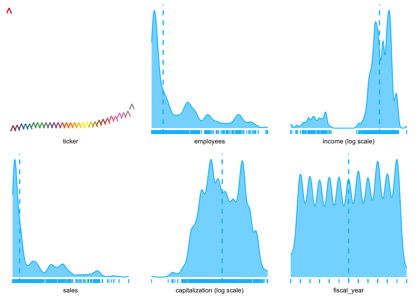
.~1 shows distribution of each variable in the data frame, separately.
industry_stats |>
  dplyr::filter(income >= 0 ) |> # filter data
  plotluck(income ~ .) # plot the data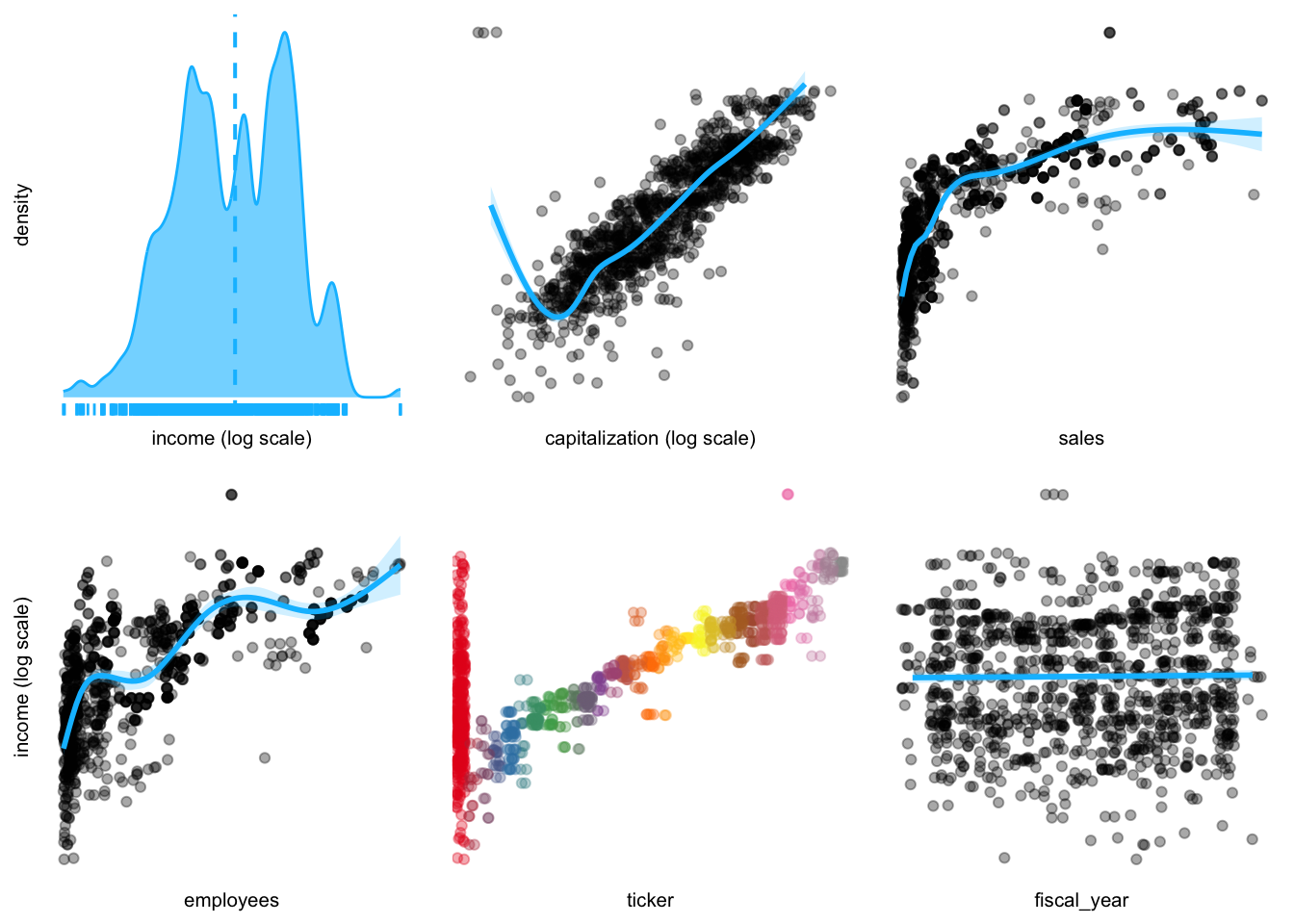
industry_stats |>
  dplyr::select(-ticker) |> # tickerを除外
  dplyr::filter(income >= 0) |> # 利益が0以上のデータ
  plotluck(income ~ .) # 作図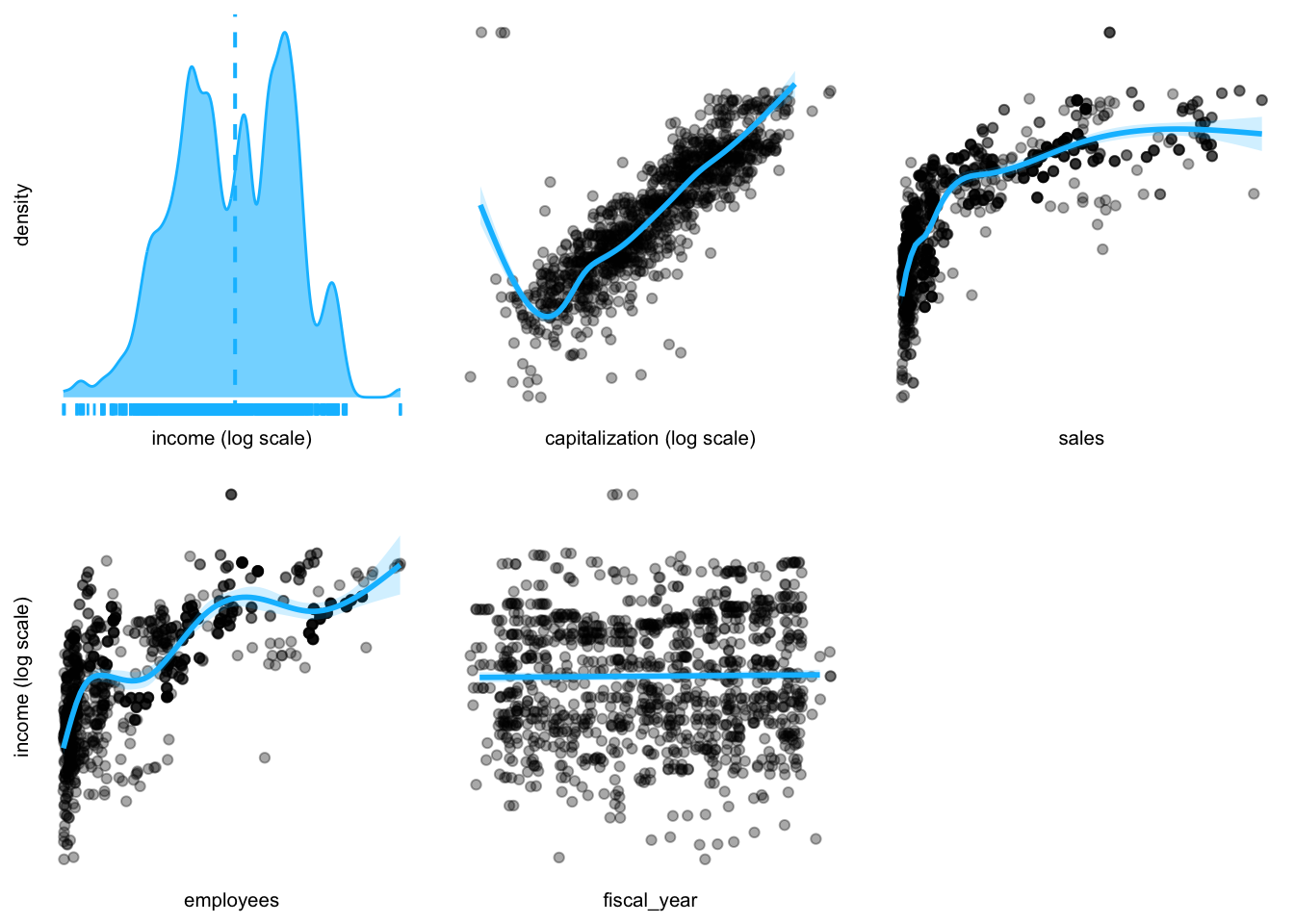
industry_stats |>
  dplyr::filter(income >= 0) |> # 利益が0以上のデータ
  plotluck(income ~ fiscal_year) # income vs fiscal year
sox_stats <- read_csv( # read csv file
    system.file(
      "extdata",
      "ch_2_data_types.csv", # dataset
      package = "auditanalytics",
      mustWork = TRUE
      )
      )


head(sox_stats)
# A tibble: 6 × 19
ticker date card disc hack insd phys port stat unkn effective_303
<chr> <dbl> <chr> <dbl> <dbl> <dbl> <dbl> <dbl> <dbl> <dbl> <dbl>
1 A 2008 0 0 0 0 0 1 0 0 1
2 A 2008 0 0 0 0 0 1 0 0 1
3 A 2008 0 0 0 0 0 1 0 0 1
4 A 2008 0 0 0 0 0 1 0 0 1
5 A 2008 0 0 0 0 0 1 0 0 1
6 AAN 2011 0 0 0 0 0 0 1 0 1
# ℹ 8 more variables: mat_weak_303 <dbl>, sig_def_303 <dbl>, auto_1 <dbl>,
# auditor_agrees_303 <dbl>, effective_404 <dbl>, audit_fee <dbl>,
# non_audit_fee <dbl>, tax_fees <dbl>summary(sox_stats) # descriptive stats ticker date card disc
Length:1514 Min. :2005 Length:1514 Min. :0.0000
Class :character 1st Qu.:2007 Class :character 1st Qu.:0.0000
Mode :character Median :2010 Mode :character Median :0.0000
Mean :2010 Mean :0.1739
3rd Qu.:2013 3rd Qu.:0.0000
Max. :2016 Max. :1.0000
NA's :2 NA's :2
hack insd phys port
Min. :0.0000 Min. :0.0000 Min. :0.0000 Min. :0.0000
1st Qu.:0.0000 1st Qu.:0.0000 1st Qu.:0.0000 1st Qu.:0.0000
Median :0.0000 Median :0.0000 Median :0.0000 Median :0.0000
Mean :0.2467 Mean :0.1382 Mean :0.0463 Mean :0.2837
3rd Qu.:0.0000 3rd Qu.:0.0000 3rd Qu.:0.0000 3rd Qu.:1.0000
Max. :1.0000 Max. :1.0000 Max. :1.0000 Max. :1.0000
NA's :2 NA's :2 NA's :2 NA's :2
stat unkn effective_303 mat_weak_303
Min. :0.00000 Min. :0.00000 Min. :0.0000 Min. :0.00000
1st Qu.:0.00000 1st Qu.:0.00000 1st Qu.:1.0000 1st Qu.:0.00000
Median :0.00000 Median :0.00000 Median :1.0000 Median :0.00000
Mean :0.03704 Mean :0.03968 Mean :0.9616 Mean :0.03241
3rd Qu.:0.00000 3rd Qu.:0.00000 3rd Qu.:1.0000 3rd Qu.:0.00000
Max. :1.00000 Max. :1.00000 Max. :1.0000 Max. :1.00000
NA's :2 NA's :2 NA's :2 NA's :2
sig_def_303 auto_1 auditor_agrees_303 effective_404
Min. :0.0000 Min. :0.0000 Min. :0.00000 Min. :0.0000
1st Qu.:0.0000 1st Qu.:0.0000 1st Qu.:0.00000 1st Qu.:0.0000
Median :0.0000 Median :0.0000 Median :0.00000 Median :0.0000
Mean :0.1157 Mean :0.2037 Mean :0.08003 Mean :0.3935
3rd Qu.:0.0000 3rd Qu.:0.0000 3rd Qu.:0.00000 3rd Qu.:1.0000
Max. :1.0000 Max. :1.0000 Max. :1.00000 Max. :1.0000
NA's :2 NA's :2 NA's :2 NA's :2
audit_fee non_audit_fee tax_fees
Min. : 100000 Min. : 0 Min. : 0
1st Qu.: 3785984 1st Qu.: 477686 1st Qu.: 93140
Median : 7956000 Median : 1068000 Median : 370000
Mean : 15321536 Mean : 3679039 Mean : 1451705
3rd Qu.: 17800000 3rd Qu.: 3400000 3rd Qu.: 1311000
Max. :112200000 Max. :41100000 Max. :20800000
NA's :2 NA's :2 NA's :2 make histogram
sox_stats |> # choose the variables
    ggplot() +  # プラスの直後で改行OK
    aes(x = audit_fee) +  # 変数を指定
    geom_histogram(bins = 20) # ヒストグラム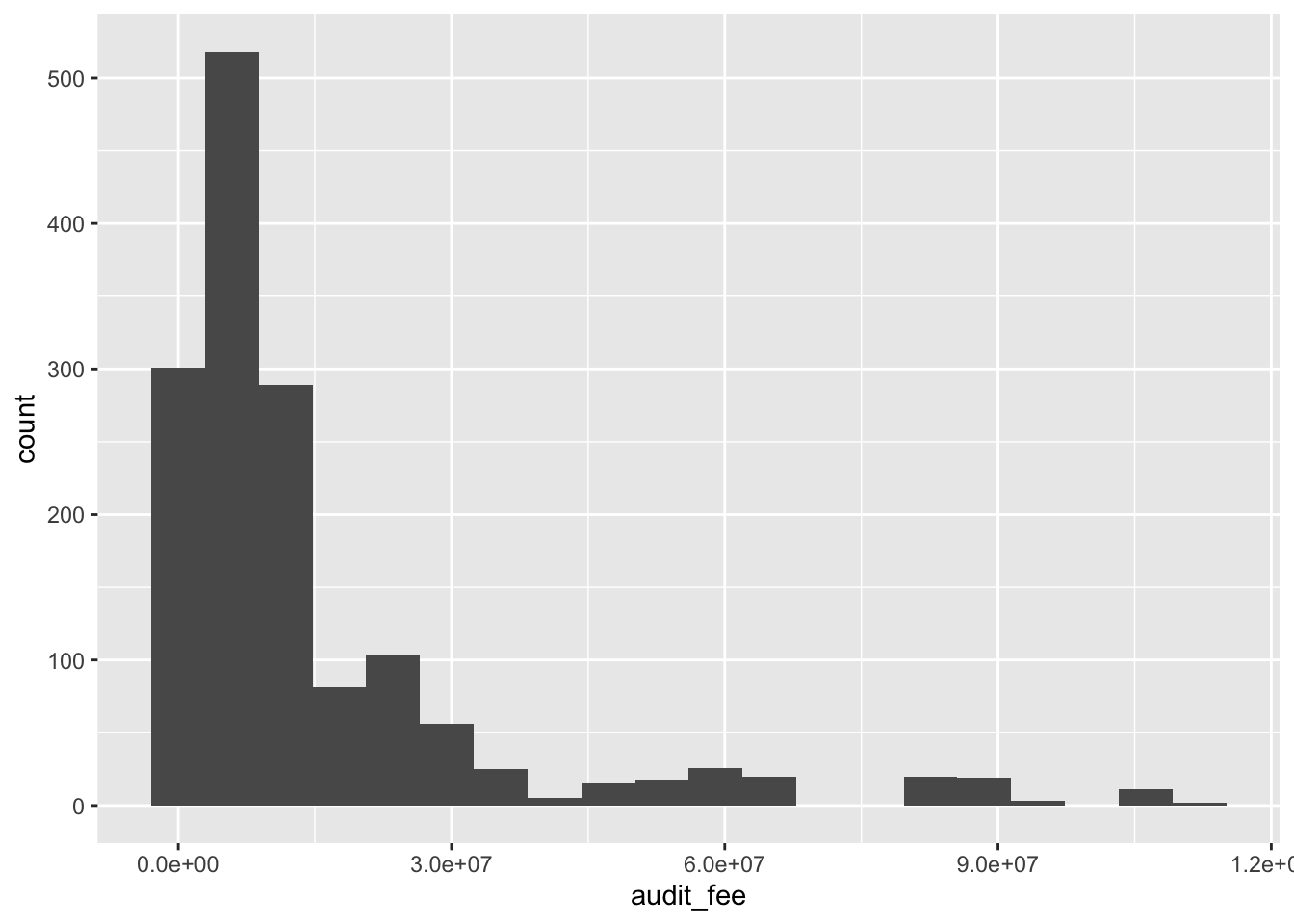
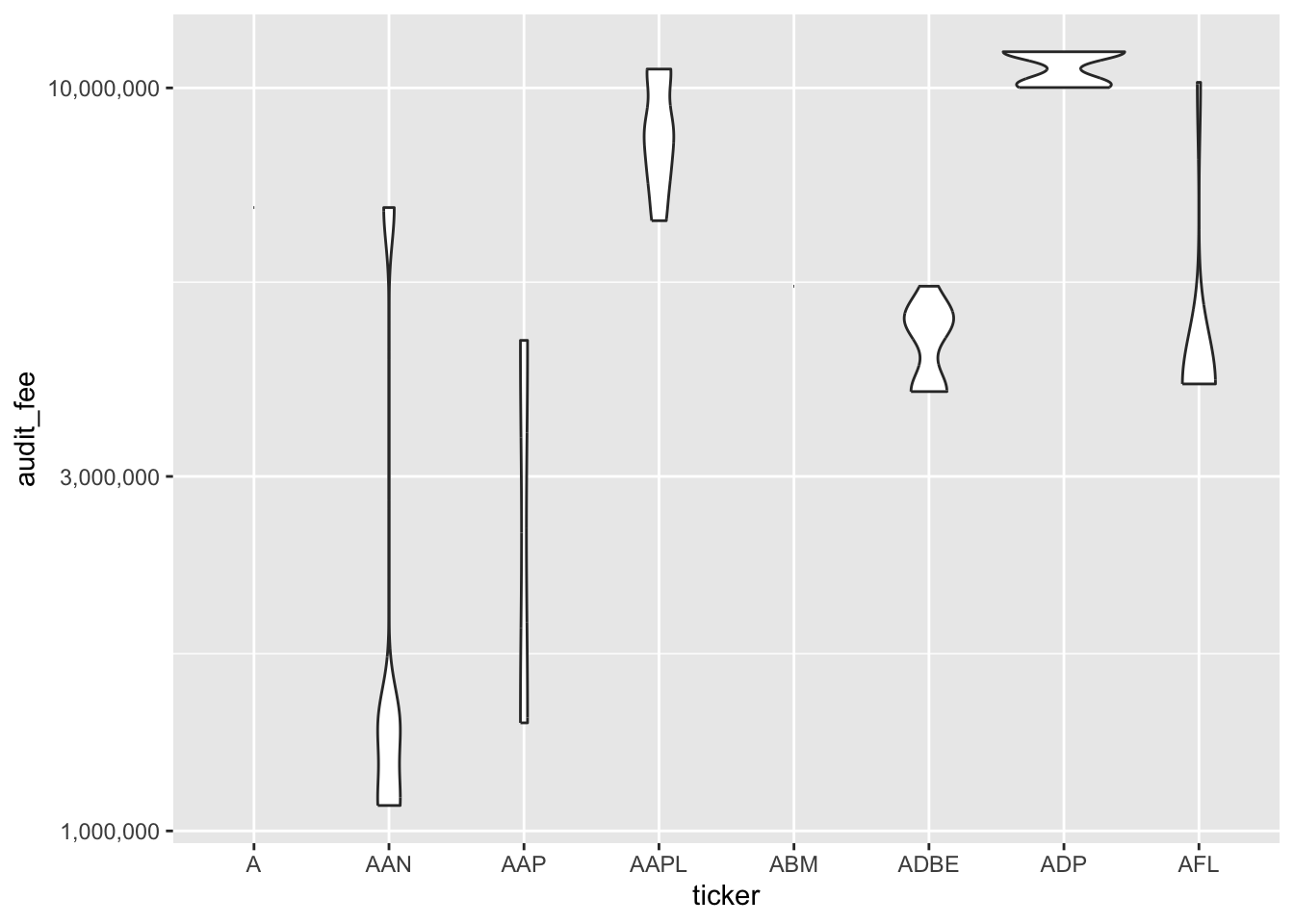
Categorical Data
sox_stats |>
  filter(as.character(ticker) < "AI") |> # data before "AI"
  ggplot() +
  aes(x = ticker, y = audit_fee) + # 軸の指定
  geom_violin() + # violin plot
  scale_y_continuous(
    trans = "log10", # 常用対数
    labels = scales::comma # comma format
    )
bank_fin <- read_csv( # CSVファイルを読み込む
  system.file(
    "extdata",
    "ch_2_yahoo_fin.csv", # データセット
    package = "auditanalytics",
    mustWork = TRUE
    )
  )

head(bank_fin)
# A tibble: 6 × 9
ticker name price change percent_change volume vol_ave capitalization
<chr> <chr> <dbl> <chr> <dbl> <dbl> <dbl> <chr>
1 HSBC-PA HSBC Holdi… 2.65e1 0.00 0 2.64e4 6.15e4 541.154B
2 BRK-B Berkshire … 2.01e2 1.92 0.97 2.02e6 3.78e6 493.498B
3 BRK-A Berkshire … 3.02e5 2631.… 0.88 2.43e2 2.45e2 492.962B
4 V Visa Inc. 1.80e2 -0.87 -0.48 3.59e6 6.91e6 403.496B
5 JPM JPMorgan C… 1.09e2 1.10 1.02 6.51e6 1.15e7 347.679B
6 SAN-PB Banco Sant… 2.27e1 0.04 0.18 1.20e4 1.94e4 349.445B
# ℹ 1 more variable: pe_ratio <dbl>bank_fin |>
filter(change != "ticker") |> # ticker以外
mutate(# データの変換
change = as.numeric(change), # 数値に変換
capitalization = as.numeric( # Bを削除
str_replace(capitalization, "B", "")
)
) |>
pivot_longer( # wide to long
cols = c(price, change, percent_change, volume,
vol_ave, capitalization, pe_ratio),
names_to = "metric", # 変数名
values_to = "value" # 値
) |>
ggplot() + # 作図
aes(x = metric, y = value) + # 軸の指定
geom_boxplot() + # 箱ひげ図
scale_y_continuous(
trans = "log10",
labels = scales::comma
) # 縦軸を対数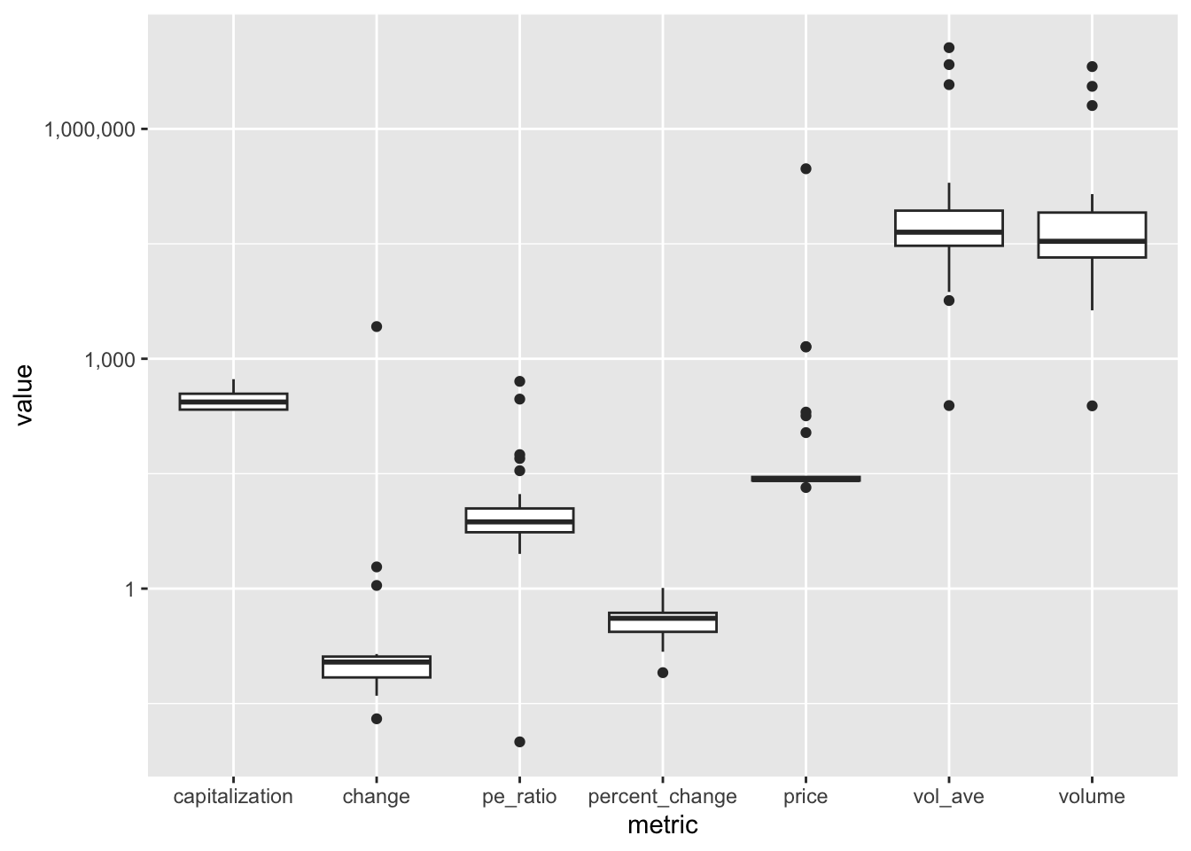
Binary Data
ggplot(sox_stats) +
    aes(x = non_audit_fee, y = audit_fee, col = card) + # 軸と色分け
    geom_violin() + # ヴァイオリンプロット
    labs(col = "Fraud = 1 (green)") + # 軸ラベル
    scale_y_continuous(labels = scales::comma) +
    scale_x_continuous(labels = scales::comma)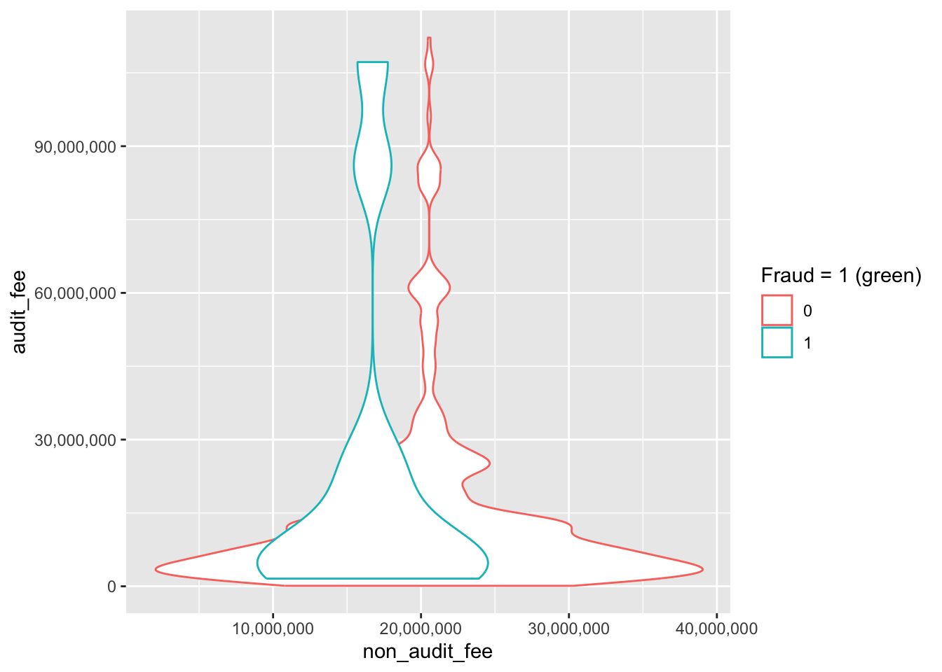
整数に変換 as.integer()
sox_stats$card <- as.integer(sox_stats$card)

sox_stats_long <- sox_stats |>
  pivot_longer( # wide to long
    cols = c(effective_303, mat_weak_303, sig_def_303,
             effective_404, auditor_agrees_303),
    names_to = "metric", # 変数名
    values_to = "value") # 値

# 作図
ggplot(sox_stats_long) +
    aes(x = non_audit_fee, y = audit_fee, col = metric) +
    geom_violin() + # バイオリン・プロット
    scale_x_continuous(trans = "log2", labels = scales::comma) +
    scale_y_continuous(trans = "log2", labels = scales::comma) # 対数軸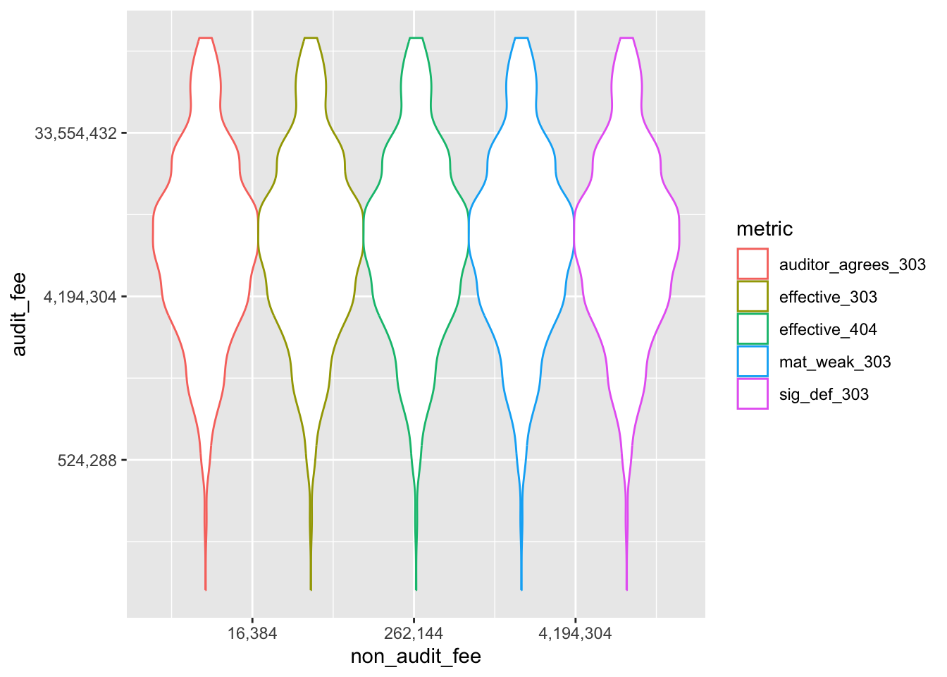
Make an original function
rdate <- function( # 引数を指定
    x,
    min = paste0(format(Sys.Date(), "%Y"), "-01-01"),
    max = paste0(format(Sys.Date(), "%Y"), "-12-31"),
    sort = TRUE
    ) { # 関数の本体
    dates <- sample(
        seq(as.Date(min), as.Date(max), by = "day"),
        x, replace = TRUE)
    if (sort == TRUE) {
        return(sort(dates))
    } else {
        return(dates)
    }
}

journal_ent_no <- tibble( # data.frameを作成
  date = rdate(1000), # ランダムな日付
  invoice_no = seq(1, 1000) + rbinom(1000, 1, 0.1) # 請求書番号
) |>
  arrange(date) |> # 日付で並び替え
  mutate( # 重複する日付をマーク
    invoice_no = if_else(duplicated(invoice_no), NA, invoice_no),
    duplicates = duplicated(invoice_no) # duplicates
  )

journal_dups <- journal_ent_no |>
  mutate(
    raw = row_number(), # row number
    duplicates = duplicated(invoice_no) # duplicates
    )

glimpse(journal_dups)
Rows: 1,000
Columns: 4
$ date <date> 2024-01-01, 2024-01-01, 2024-01-01, 2024-01-01, 2024-01-02…
$ invoice_no <int> 1, 2, 3, 4, 5, 6, 7, 8, 9, 10, 11, 12, 13, 14, 15, 16, 17, …
$ duplicates <lgl> FALSE, FALSE, FALSE, FALSE, FALSE, FALSE, FALSE, FALSE, FAL…
$ raw <int> 1, 2, 3, 4, 5, 6, 7, 8, 9, 10, 11, 12, 13, 14, 15, 16, 17, …table(journal_dups$duplicates)
FALSE  TRUE
919 81 ggplot(journal_dups) +
aes(x = invoice_no, y = raw,
shape = duplicates, color = duplicates) +
geom_point() # 散布図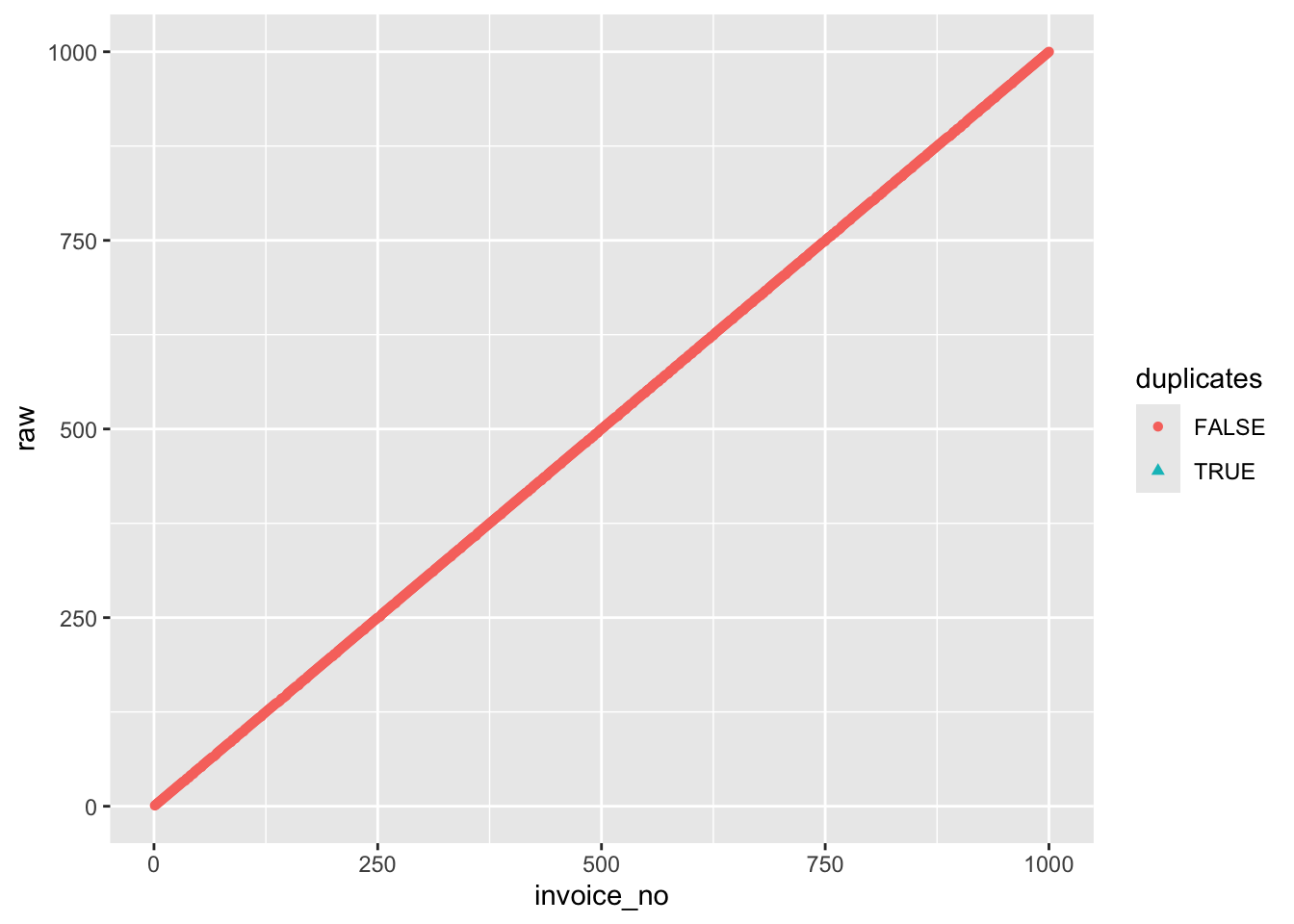
journal_ent_no |>
  filter(duplicates == TRUE, invoice_no < 100) |>
  kable(longtable = T, caption = "Duplicated Invoices") |>
  kable_styling(
    bootstrap_options = c("striped", "hover", "condensed"),
full_width = F, font_size = 20)| date | invoice_no | duplicates |
|---|---|---|
| NA | NA | NA |
| :---- | ----------: | :---------- |
journal_dups <- journal_dups |>
  mutate(
    invoice = journal_ent_no$invoice_no,
    omit = !raw %in% journal_ent_no$invoice
  )


glimpse(journal_dups)
Rows: 1,000
Columns: 6
$ date <date> 2024-01-01, 2024-01-01, 2024-01-01, 2024-01-01, 2024-01-02…
$ invoice_no <int> 1, 2, 3, 4, 5, 6, 7, 8, 9, 10, 11, 12, 13, 14, 15, 16, 17, …
$ duplicates <lgl> FALSE, FALSE, FALSE, FALSE, FALSE, FALSE, FALSE, FALSE, FAL…
$ raw <int> 1, 2, 3, 4, 5, 6, 7, 8, 9, 10, 11, 12, 13, 14, 15, 16, 17, …
$ invoice <int> 1, 2, 3, 4, 5, 6, 7, 8, 9, 10, 11, 12, 13, 14, 15, 16, 17, …
$ omit <lgl> TRUE, TRUE, TRUE, TRUE, TRUE, TRUE, TRUE, TRUE, TRUE, TRUE,…ggplot(journal_dups) +
aes(x = invoice_no, y = raw, col = omit) +
geom_point() + labs(col = "Invoice Omitted?")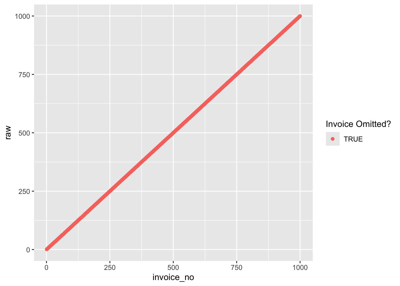
Big Data
big_data <- read_csv(
  system.file(
    "extdata",
    "ch1_amount_data.csv",
    package = "auditanalytics",
    mustWork = TRUE
    )
  ) |>
  pivot_longer(# wide to long
    cols = c(-year),
    names_to = "data_type",
    values_to = "value"
    )
head(big_data)
# A tibble: 6 × 3
year data_type value
<dbl> <chr> <dbl>
1 1930 transient 0
2 1930 financial 323436613.
3 1930 text 332755554.
4 1930 multimedia 0
5 1930 mobile 0
6 1932 transient 0 big_data$amount <- sqrt(big_data$value)
big_data %>%
ggplot() + aes(x = year, y = amount, col=data_type) +
geom_point(aes(color = data_type, size = amount), alpha = 0.5) +
scale_size(range = c(0.5, 12)) +
scale_y_continuous(trans = "sqrt") +
xlim(1990,2020) + xlab("Year") +
ylab("Number of Bits of Storage")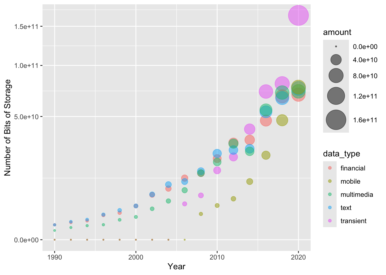
Vectors
a <- c(1, 2, 5.3, 6, -2, 4) # number vector
b <- c("one", "two", "three") # character vector
c <- c(TRUE,TRUE,TRUE,FALSE,TRUE,FALSE) # logical vector

a[c(2,4)] # 2nd and 4th elements of the vector
[1] 2 6Matrix
sequence of numbers from 1 to 25
vector <- seq(1, 25)
r <- 5
c <- 5

mat <- matrix(vector,
  nrow = r, # row
  ncol = c, # column
  byrow = FALSE # 行と列を入れ替えない
  )

print(mat) # 行列を表示
[,1] [,2] [,3] [,4] [,5]
[1,] 1 6 11 16 21
[2,] 2 7 12 17 22
[3,] 3 8 13 18 23
[4,] 4 9 14 19 24
[5,] 5 10 15 20 25Try this code
Indexing
# 5行4列の行列を作成
y <- matrix(1:20, nrow=5,ncol=4)
y
[,1] [,2] [,3] [,4]
[1,] 1 6 11 16
[2,] 2 7 12 17
[3,] 3 8 13 18
[4,] 4 9 14 19
[5,] 5 10 15 20# another example
cells <- c(1,26,24,68)
rnames <- c("R1", "R2")
cnames <- c("C1", "C2")
mymatrix <- matrix(cells,
nrow = 2,
ncol = 2,
byrow = TRUE,
dimnames = list(rnames, cnames)
)
mymatrix C1 C2
R1 1 26
R2 24 68mat[, 4] # 4th column of the matrix[1] 16 17 18 19 20mat[3,] # 3rd row of the matrix[1] 3 8 13 18 23mat[2:4,1:3] # rows 2 to 4 and columns 1 to 3 [,1] [,2] [,3]
[1,] 2 7 12
[2,] 3 8 13
[3,] 4 9 14set.seed(123) # set seed for reproducibility
x <- sample(1:20, 9) # 9 random numbers
mat <- matrix(x, nrow = 3, ncol = 3) # 3x3 matrix
print(mat) # print the matrix [,1] [,2] [,3]
[1,] 15 3 6
[2,] 19 10 11
[3,] 14 2 5## Inverse Matrix
solve(mat) [,1] [,2] [,3]
[1,] -1.866667 0.2 1.8
[2,] -3.933333 0.6 3.4
[3,] 6.800000 -0.8 -6.2## Unit Matrix
mat %*% solve(mat) |> round(5) # unit matrix [,1] [,2] [,3]
[1,] 1 0 0
[2,] 0 1 0
[3,] 0 0 1Create a data frame
ID <- c(1, 2, 3, 4) # numeric vector
Color <- c("red", "white", "red", NA) # character vector
Passed <- c(TRUE, TRUE, TRUE, FALSE) # logical vector

mydata <- data.frame(ID, Color, Passed) # create data frame
# access elements of the data frame
mydata[1:2] # columns 1 and 2 of data frame
ID Color
1 1 red
2 2 white
3 3 red
4 4 <NA>mydata[c("ID","Color")] # columns ID and Age from data frame ID Color
1 1 red
2 2 white
3 3 red
4 4 <NA>## Example: Data Frame
mydata <- data.frame(
ID = c(1, 2, 3, 4),
Color = c("red", "white", "red", NA),
Passed = c(TRUE, TRUE, TRUE, FALSE)
)
# mydataからColorを取り出す
mydata["Color"] Color
1 red
2 white
3 red
4 <NA># mydataからIDの3番目の要素を取り出す
mydata[3,"ID"][1] 3List
a <- b <- "seven"
z <- y <- 0
# example of a list with 4 components -
w <- list(name = "Fred", mynumbers = a, mymatrix = y, age = 5.3)
w
$name
[1] "Fred"
$mynumbers
[1] "seven"
$mymatrix
[1] 0
$age
[1] 5.3list1 <- list(name = "Fred", mynumbers = a, mymatrix = y, age = 5.3)
list2 <- list(name = "Joe", mynumbers = b, mymatrix = z, age = 10.11) # 誤字
v <- c(list1,list2)
v$name
[1] "Fred"
$mynumbers
[1] "seven"
$mymatrix
[1] 0
$age
[1] 5.3
$name
[1] "Joe"
$mynumbers
[1] "seven"
$mymatrix
[1] 0
$age
[1] 10.11w[[1]] # 1st component of the list[1] "Fred"v[["mynumbers"]] # component named mynumbers in list[1] "seven"## Example: list
mylist <- list(
a <- c("one", "two", "three"),
b <- c(1,2,3),
c <- matrix(1:9, nrow = 3)
)
# mylistからaを取り出す
mylist[1][[1]]
[1] "one" "two" "three"# mylistからbの2番目の要素を取り出す
mylist[[2]][2][1] 2factor
gender <- c(rep("male", 20), rep("female", 30))
gender <- factor(gender) # ファクター型に変換
gender
[1] male male male male male male male male male male
[11] male male male male male male male male male male
[21] female female female female female female female female female female
[31] female female female female female female female female female female
[41] female female female female female female female female female female
Levels: female malesummary(gender)female male
30 20 rating <- c("medium", "large", "small") # 文字ベクトル
rating <- ordered(rating, levels = c("small", "medium", "large"))
rating[1] medium large small
Levels: small < medium < largearry <- read_csv( #
system.file(
"extdata",
"morph_array.csv", #
package = "auditanalytics",
mustWork = TRUE
)
)
head(arry)# A tibble: 5 × 11
scope ben_1 cost_1 ben_2 cost_2 ben_3 cost_3 ben_4 cost_4 ben_5 cost_5
<dbl> <dbl> <dbl> <dbl> <dbl> <dbl> <dbl> <dbl> <dbl> <dbl> <dbl>
1 1 810 500 940 440 140 130 190 170 20 10
2 2 1370 890 1610 1010 3970 2770 3430 2460 3020 2650
3 3 9070 4850 6190 3250 5710 3590 7650 5360 7970 5220
4 4 4720 2400 4650 3950 330 260 2120 1580 2600 2020
5 5 8650 4830 9100 4060 5090 3480 8400 7540 5930 4610arry |>
kable(longtable = T) |>
kable_styling( # specify table style
bootstrap_options = c("striped", "hover", "condensed"),
full_width = F, font_size = 18
)| scope | ben_1 | cost_1 | ben_2 | cost_2 | ben_3 | cost_3 | ben_4 | cost_4 | ben_5 | cost_5 |
|---|---|---|---|---|---|---|---|---|---|---|
| 1 | 810 | 500 | 940 | 440 | 140 | 130 | 190 | 170 | 20 | 10 |
| 2 | 1370 | 890 | 1610 | 1010 | 3970 | 2770 | 3430 | 2460 | 3020 | 2650 |
| 3 | 9070 | 4850 | 6190 | 3250 | 5710 | 3590 | 7650 | 5360 | 7970 | 5220 |
| 4 | 4720 | 2400 | 4650 | 3950 | 330 | 260 | 2120 | 1580 | 2600 | 2020 |
| 5 | 8650 | 4830 | 9100 | 4060 | 5090 | 3480 | 8400 | 7540 | 5930 | 4610 |
length(arry) # 要素・コンポーネントの数[1] 11class(arry) # オブジェクトのクラス・型[1] "spec_tbl_df" "tbl_df" "tbl" "data.frame" names(arry) # オブジェクトの変数名 [1] "scope" "ben_1" "cost_1" "ben_2" "cost_2" "ben_3" "cost_3" "ben_4"
[9] "cost_4" "ben_5" "cost_5"Chapter 3. Analysis of Accounting Transactions
lubridate packages
pacman::p_load(auditanalytics, tidyverse)lubridate is a package that makes it easier to work with dates and times in R.
ymd(20101215) # year month day[1] "2010-12-15"mdy("4/1/17") # month day year[1] "2017-04-01"bday <- dmy("14/10/1979")
month(bday) # 月を取得[1] 10wday(bday, label = TRUE) # 1979年10月14日は日曜日[1] 日
Levels: 日 < 月 < 火 < 水 < 木 < 金 < 土year(bday) <- 2016
wday(bday, label = TRUE) # 2016年10月14日は金曜日[1] 金
Levels: 日 < 月 < 火 < 水 < 木 < 金 < 土Accounting Transactions for Auditors
price <- rpois(n = 1000, lambda = 2)  # ポワソン分布から1000個の乱数を生成
price |> head()
[1] 5 2 3 2 0 4quantity <- rpois(1000, 10000) # ポワソン分布から1000個の乱数を生成
quantity |> head()[1] 9990 10001 10075 10036 9941 10021value <- price * quantity # 価格と数量の積
qplot(value, geom = "histogram") # ヒストグラム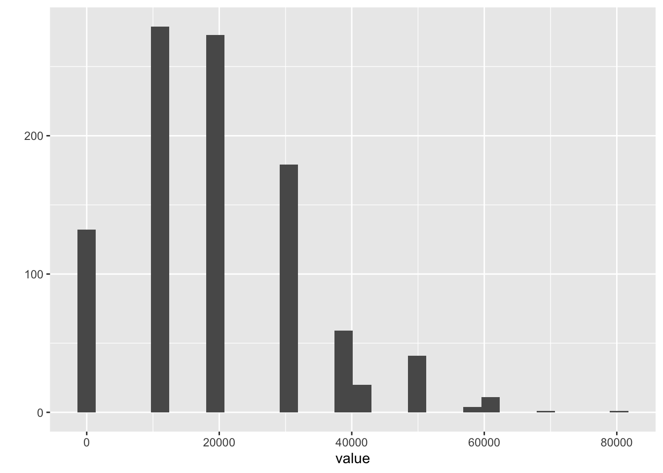
qplot(value, geom = "density") # 密度分布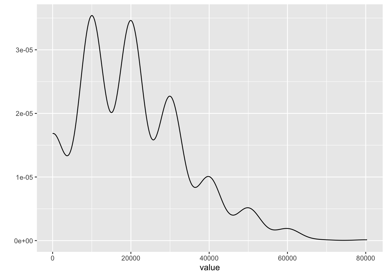
disburse <- read_csv(system.file( # csvファイルの読み込み
    "extdata",
    "ch_2_AP_disbursements_journal.csv", # ファイル名
    package = "auditanalytics",
    mustWork = TRUE
    )
  ) # ファイルがない場合はエラーを返す

summary(disburse) # descriptive statistics
disbursement_no date amount_paid
Length:50 Min. :2018-03-21 Min. :2417
Class :character 1st Qu.:2018-06-27 1st Qu.:2537
Mode :character Median :2018-10-12 Median :2618
Mean :2018-10-07 Mean :2686
3rd Qu.:2018-12-24 3rd Qu.:2800
Max. :2019-06-20 Max. :3190 # output the total amount paid
cat('\n\n 支払帳の合計金額 = ', sum(disburse$amount_paid))
支払帳の合計金額 = 134313.5library(Hmisc) # 記述統計量の計算
bank_fin <- read.csv(system.file(
"extdata",
"ch_2_yahoo_fin.csv",
package = "auditanalytics",
mustWork = TRUE
)
)
Hmisc::describe(bank_fin) # Show summary statisticsbank_fin
9 Variables 38 Observations
--------------------------------------------------------------------------------
ticker
n missing distinct
25 13 25
lowest : BAC-PC BAC-PE BAC-PK BAC-PL BAC-PY, highest: WFC-PR WFC-PV WFC-PW WFC-PX WFC-PY
--------------------------------------------------------------------------------
name
n missing distinct
25 13 7
lowest : Banco Santander, S.A. GTD PFD SECS 6 Bank of America Corporation Berkshire Hathaway Inc. HSBC Holdings plc ADR A 1/40PF A JPMorgan Chase & Co.
highest: Berkshire Hathaway Inc. HSBC Holdings plc ADR A 1/40PF A JPMorgan Chase & Co. Visa Inc. Wells Fargo & Company
--------------------------------------------------------------------------------
price
n missing distinct Info Mean Gmd .05 .10
25 13 25 1 12231 24374 22.38 22.93
.25 .50 .75 .90 .95
25.70 26.45 28.66 935.15 1437.69
Value 0e+00 3e+05
Frequency 24 1
Proportion 0.96 0.04
For the frequency table, variable is rounded to the nearest 5000
--------------------------------------------------------------------------------
change
n missing distinct
26 12 22
lowest : -0.01 -0.03 -0.04 -0.06 -0.07
highest: 0.14 1.10 1.92 2631.00 ticker
--------------------------------------------------------------------------------
percent_change
n missing distinct Info Mean Gmd .05 .10
25 13 23 0.999 0.2016 0.4513 -0.268 -0.252
.25 .50 .75 .90 .95
-0.110 0.180 0.410 0.740 0.952
lowest : -0.48 -0.27 -0.26 -0.24 -0.19, highest: 0.44 0.53 0.88 0.97 1.02
--------------------------------------------------------------------------------
volume
n missing distinct Info Mean Gmd .05 .10
25 13 25 1 520349 939507 4340 5020
.25 .50 .75 .90 .95
20982 34142 80933 1267169 3278800
lowest : 243 4284 4566 5700 11997
highest: 89764 140922 2018000 3594000 6506000
--------------------------------------------------------------------------------
vol_ave
n missing distinct Info Mean Gmd .05 .10
25 13 25 1 935629 1706024 6093 7569
.25 .50 .75 .90 .95
29831 44849 85711 2347830 6281000
Value 0 100000 3700000 6900000 11400000
Frequency 19 3 1 1 1
Proportion 0.76 0.12 0.04 0.04 0.04
For the frequency table, variable is rounded to the nearest 100000
--------------------------------------------------------------------------------
capitalization
n missing distinct
25 13 25
lowest : 211.288B 212.921B 214.807B 215.543B 216.366B
highest: 368.674B 403.496B 492.962B 493.498B 541.154B
--------------------------------------------------------------------------------
pe_ratio
n missing distinct Info Mean Gmd .05 .10
25 13 25 1 43.2 71.1 2.846 3.834
.25 .50 .75 .90 .95
5.440 7.430 11.120 53.596 249.240
Value 0 5 10 15 30 45 55 295 505
Frequency 3 15 1 1 1 1 1 1 1
Proportion 0.12 0.60 0.04 0.04 0.04 0.04 0.04 0.04 0.04
For the frequency table, variable is rounded to the nearest 5
--------------------------------------------------------------------------------library(psych) # 心理統計学のためのパッケージ
psych::describe(bank_fin) # 記述統計量の出力 vars n mean sd median trimmed mad min
ticker* 1 38 9.55 8.61 7.50 8.91 9.64 1.00
name* 2 38 4.05 2.89 3.00 3.97 2.97 1.00
price 3 25 12231.23 60356.40 26.45 112.41 1.93 20.88
change* 4 38 8.84 7.52 7.50 8.34 9.64 1.00
percent_change 5 25 0.20 0.39 0.18 0.18 0.37 -0.48
volume 6 25 520348.92 1480580.79 34142.00 138295.05 32832.18 243.00
vol_ave 7 25 935628.64 2678595.35 44849.00 237653.14 45797.51 245.00
capitalization* 8 38 9.55 8.61 7.50 8.91 9.64 1.00
pe_ratio 9 25 43.20 113.07 7.43 12.99 3.16 0.01
max range skew kurtosis se
ticker* 26.00 25.00 0.47 -1.30 1.40
name* 8.00 7.00 0.30 -1.61 0.47
price 301936.00 301915.12 4.42 18.23 12071.28
change* 23.00 22.00 0.37 -1.40 1.22
percent_change 1.02 1.50 0.41 -0.63 0.08
volume 6506000.00 6505757.00 3.01 8.48 296116.16
vol_ave 11488000.00 11487755.00 2.90 7.68 535719.07
capitalization* 26.00 25.00 0.47 -1.30 1.40
pe_ratio 506.93 506.92 3.19 9.35 22.61psych::describeBy(bank_fin, bank_fin$name)
 Descriptive statistics by group
group:
               vars  n mean  sd median trimmed mad min  max range skew kurtosis
ticker            1 13 1.00 0.0      1       1   0   1    1     0  NaN      NaN
name              2 13 1.00 0.0      1       1   0   1    1     0  NaN      NaN
price             3  0  NaN  NA     NA     NaN  NA Inf -Inf  -Inf   NA       NA
change            4 13 2.69 6.1      1       1   0   1   23    22 2.82     6.44
percent_change    5  0  NaN  NA     NA     NaN  NA Inf -Inf  -Inf   NA       NA
volume            6  0  NaN  NA     NA     NaN  NA Inf -Inf  -Inf   NA       NA
vol_ave           7  0  NaN  NA     NA     NaN  NA Inf -Inf  -Inf   NA       NA
capitalization    8 13 1.00 0.0      1       1   0   1    1     0  NaN      NaN
pe_ratio          9  0  NaN  NA     NA     NaN  NA Inf -Inf  -Inf   NA       NA
                 se
ticker         0.00
name           0.00
price            NA
change         1.69
percent_change   NA
volume           NA
vol_ave          NA
capitalization 0.00
pe_ratio         NA
------------------------------------------------------------
group: Banco Santander, S.A. GTD PFD SECS 6
               vars n     mean sd   median  trimmed mad      min      max range
ticker            1 1    15.00 NA    15.00    15.00   0    15.00    15.00     0
name              2 1     2.00 NA     2.00     2.00   0     2.00     2.00     0
price             3 1    22.72 NA    22.72    22.72   0    22.72    22.72     0
change            4 1    12.00 NA    12.00    12.00   0    12.00    12.00     0
percent_change    5 1     0.18 NA     0.18     0.18   0     0.18     0.18     0
volume            6 1 11997.00 NA 11997.00 11997.00   0 11997.00 11997.00     0
vol_ave           7 1 19388.00 NA 19388.00 19388.00   0 19388.00 19388.00     0
capitalization    8 1    20.00 NA    20.00    20.00   0    20.00    20.00     0
pe_ratio          9 1    49.93 NA    49.93    49.93   0    49.93    49.93     0
               skew kurtosis se
ticker           NA       NA NA
name             NA       NA NA
price            NA       NA NA
change           NA       NA NA
percent_change   NA       NA NA
volume           NA       NA NA
vol_ave          NA       NA NA
capitalization   NA       NA NA
pe_ratio         NA       NA NA
------------------------------------------------------------
group: Bank of America Corporation
               vars n     mean       sd   median  trimmed      mad     min
ticker            1 7     5.00     2.16     5.00     5.00     2.97    2.00
name              2 7     3.00     0.00     3.00     3.00     0.00    3.00
price             3 7   224.31   529.23    25.78   224.31     3.77   20.88
change            4 7     6.43     4.31     5.00     6.43     2.97    3.00
percent_change    5 7    -0.11     0.24    -0.19    -0.11     0.12   -0.27
volume            6 7 33409.00 29580.81 32345.00 33409.00 32341.44 4566.00
vol_ave           7 7 41777.29 34055.28 29831.00 41777.29 35695.08 5755.00
capitalization    8 7    15.00     2.16    15.00    15.00     2.97   12.00
pe_ratio          9 7    79.83   188.34     9.17    79.83     1.33    7.43
                    max    range skew kurtosis       se
ticker             8.00     6.00 0.00    -1.71     0.82
name               3.00     0.00  NaN      NaN     0.00
price           1424.47  1403.59 1.62     0.80   200.03
change            15.00    12.00 0.98    -0.63     1.63
percent_change     0.41     0.68 1.37     0.28     0.09
volume         86124.00 81558.00 0.56    -1.25 11180.50
vol_ave        85711.00 79956.00 0.18    -2.02 12871.69
capitalization    18.00     6.00 0.00    -1.71     0.82
pe_ratio         506.93   499.50 1.62     0.80    71.18
------------------------------------------------------------
group: Berkshire Hathaway Inc.
               vars n       mean         sd     median    trimmed        mad
ticker            1 2       9.50       0.71       9.50       9.50       0.74
name              2 2       4.00       0.00       4.00       4.00       0.00
price             3 2  151068.58  213358.75  151068.58  151068.58  223676.04
change            4 2      21.50       0.71      21.50      21.50       0.74
percent_change    5 2       0.92       0.06       0.92       0.92       0.07
volume            6 2 1009121.50 1426769.66 1009121.50 1009121.50 1495763.26
vol_ave           7 2 1890622.50 2673397.50 1890622.50 1890622.50 2802673.68
capitalization    8 2      24.50       0.71      24.50      24.50       0.74
pe_ratio          9 2       8.57      12.11       8.57       8.57      12.70
                  min        max      range skew kurtosis         se
ticker           9.00      10.00       1.00    0    -2.75       0.50
name             4.00       4.00       0.00  NaN      NaN       0.00
price          201.16  301936.00  301734.84    0    -2.75  150867.42
change          21.00      22.00       1.00    0    -2.75       0.50
percent_change   0.88       0.97       0.09    0    -2.75       0.04
volume         243.00 2018000.00 2017757.00    0    -2.75 1008878.50
vol_ave        245.00 3781000.00 3780755.00    0    -2.75 1890377.50
capitalization  24.00      25.00       1.00    0    -2.75       0.50
pe_ratio         0.01      17.14      17.13    0    -2.75       8.56
------------------------------------------------------------
group: HSBC Holdings plc ADR A 1/40PF A
               vars n     mean sd   median  trimmed mad      min      max range
ticker            1 1    11.00 NA    11.00    11.00   0    11.00    11.00     0
name              2 1     5.00 NA     5.00     5.00   0     5.00     5.00     0
price             3 1    26.45 NA    26.45    26.45   0    26.45    26.45     0
change            4 1    10.00 NA    10.00    10.00   0    10.00    10.00     0
percent_change    5 1     0.00 NA     0.00     0.00   0     0.00     0.00     0
volume            6 1 26376.00 NA 26376.00 26376.00   0 26376.00 26376.00     0
vol_ave           7 1 61496.00 NA 61496.00 61496.00   0 61496.00 61496.00     0
capitalization    8 1    26.00 NA    26.00    26.00   0    26.00    26.00     0
pe_ratio          9 1    56.04 NA    56.04    56.04   0    56.04    56.04     0
               skew kurtosis se
ticker           NA       NA NA
name             NA       NA NA
price            NA       NA NA
change           NA       NA NA
percent_change   NA       NA NA
volume           NA       NA NA
vol_ave          NA       NA NA
capitalization   NA       NA NA
pe_ratio         NA       NA NA
------------------------------------------------------------
group: JPMorgan Chase & Co.
               vars n       mean         sd    median    trimmed      mad
ticker            1 3      13.00       1.00     13.00      13.00     1.48
name              2 3       6.00       0.00      6.00       6.00     0.00
price             3 3      54.84      46.66     28.05      54.84     0.44
change            4 3      12.67       9.45     16.00      12.67     5.93
percent_change    5 3       0.45       0.54      0.36       0.45     0.59
volume            6 3 2225376.33 3707131.82  89764.00 2225376.33 13934.96
vol_ave           7 3 3941765.67 6535296.89 198076.00 3941765.67 87258.42
capitalization    8 3      20.67       1.53     21.00      20.67     1.48
pe_ratio          9 3       5.61       4.77      2.87       5.61     0.04
                     min        max       range  skew kurtosis         se
ticker             12.00 1.4000e+01        2.00  0.00    -2.33       0.58
name                6.00 6.0000e+00        0.00   NaN      NaN       0.00
price              27.75 1.0871e+02       80.96  0.38    -2.33      26.94
change              2.00 2.0000e+01       18.00 -0.31    -2.33       5.46
percent_change     -0.04 1.0200e+00        1.06  0.16    -2.33       0.31
volume          80365.00 6.5060e+06  6425635.00  0.38    -2.33 2140313.55
vol_ave        139221.00 1.1488e+07 11348779.00  0.38    -2.33 3773155.42
capitalization     19.00 2.2000e+01        3.00 -0.21    -2.33       0.88
pe_ratio            2.84 1.1120e+01        8.28  0.38    -2.33       2.76
------------------------------------------------------------
group: Visa Inc.
               vars n       mean sd     median    trimmed mad        min
ticker            1 1      16.00 NA      16.00      16.00   0      16.00
name              2 1       7.00 NA       7.00       7.00   0       7.00
price             3 1     180.07 NA     180.07     180.07   0     180.07
change            4 1       7.00 NA       7.00       7.00   0       7.00
percent_change    5 1      -0.48 NA      -0.48      -0.48   0      -0.48
volume            6 1 3594000.00 NA 3594000.00 3594000.00   0 3594000.00
vol_ave           7 1 6906000.00 NA 6906000.00 6906000.00   0 6906000.00
capitalization    8 1      23.00 NA      23.00      23.00   0      23.00
pe_ratio          9 1      34.58 NA      34.58      34.58   0      34.58
                      max range skew kurtosis se
ticker              16.00     0   NA       NA NA
name                 7.00     0   NA       NA NA
price              180.07     0   NA       NA NA
change               7.00     0   NA       NA NA
percent_change      -0.48     0   NA       NA NA
volume         3594000.00     0   NA       NA NA
vol_ave        6906000.00     0   NA       NA NA
capitalization      23.00     0   NA       NA NA
pe_ratio            34.58     0   NA       NA NA
------------------------------------------------------------
group: Wells Fargo & Company
               vars  n     mean       sd   median  trimmed      mad     min
ticker            1 10    21.50     3.03    21.50    21.50     3.71   17.00
name              2 10     8.00     0.00     8.00     8.00     0.00    8.00
price             3 10   167.96   447.30    26.42    26.63     0.90   25.58
change            4 10    14.60     3.57    15.50    14.88     3.71    8.00
percent_change    5 10     0.29     0.19     0.36     0.31     0.15   -0.07
volume            6 10 44811.50 39786.63 32546.00 37863.62 16703.71 4284.00
vol_ave           7 10 50484.90 35897.76 39847.00 44781.88 14567.29 7758.00
capitalization    8 10     6.50     3.03     6.50     6.50     3.71    2.00
pe_ratio          9 10    34.68    92.36     5.46     5.50     0.19    5.28
                     max     range  skew kurtosis       se
ticker             26.00      9.00  0.00    -1.56     0.96
name                8.00      0.00   NaN      NaN     0.00
price            1441.00   1415.42  2.28     3.57   141.45
change             19.00     11.00 -0.42    -1.31     1.13
percent_change      0.53      0.60 -0.56    -1.13     0.06
volume         140922.00 136638.00  1.31     0.62 12581.64
vol_ave        138836.00 131078.00  1.31     0.92 11351.87
capitalization     11.00      9.00  0.00    -1.56     0.96
pe_ratio 297.54 292.26 2.28 3.57 29.21pacman::p_load(kableExtra, broom, pastecs) # パッケージの読み込み
## Tidy these up and write them as a formated table, using kableExtra
pastecs::stat.desc(bank_fin) |> # 記述統計量の計算
broom::tidy() |> # データフレームに変換
kable(longtable = T, caption = "Summary Statistics") |>
kable_styling(full_width = F, font_size = 18)| column | n | mean | sd | median | trimmed | mad | min | max | range | skew | kurtosis | se |
|---|---|---|---|---|---|---|---|---|---|---|---|---|
| ticker | 0 | NaN | NA | NA | NaN | NA | Inf | -Inf | -Inf | NA | NA | NA |
| name | 0 | NaN | NA | NA | NaN | NA | Inf | -Inf | -Inf | NA | NA | NA |
| price | 14 | 2.602796e+08 | 9.735837e+08 | 1.215125e+04 | 8.494124e+04 | 1.214879e+04 | 0.00 | 3.642895e+09 | 3.642895e+09 | 3.328201 | 12.076923 | 2.602012e+08 |
| change | 0 | NaN | NA | NA | NaN | NA | Inf | -Inf | -Inf | NA | NA | NA |
| percent_change | 14 | 3.515023e+00 | 7.098547e+00 | 6.972503e-01 | 2.057527e+00 | 5.799849e-01 | -0.48 | 2.500000e+01 | 2.548000e+01 | 2.331536 | 7.251627 | 1.897167e+00 |
| volume | 14 | 1.565820e+11 | 5.858680e+11 | 4.082325e+05 | 2.413592e+06 | 4.082246e+05 | 0.00 | 2.192119e+12 | 2.192119e+12 | 3.328201 | 12.076923 | 1.565798e+11 |
| vol_ave | 14 | 5.124946e+11 | 1.917564e+12 | 7.356739e+05 | 4.305602e+06 | 7.356659e+05 | 0.00 | 7.174873e+12 | 7.174873e+12 | 3.328201 | 12.076923 | 5.124906e+11 |
| capitalization | 0 | NaN | NA | NA | NaN | NA | Inf | -Inf | -Inf | NA | NA | NA |
| pe_ratio | 14 | 1.082288e+03 | 3.382558e+03 | 3.410240e+01 | 1.972988e+02 | 3.278888e+01 | 0.00 | 1.278445e+04 | 1.278445e+04 | 3.280235 | 11.874574 | 9.040266e+02 |
QQ-Plot
disburse <- readr::read_csv(system.file(
    "extdata",
    "ch_2_AP_disbursements_journal.csv", # csv file
    package = "auditanalytics",
    mustWork = TRUE
    )
    )

head(disburse)
# A tibble: 6 × 3
disbursement_no date amount_paid
<chr> <date> <dbl>
1 dis00001 2018-03-21 2883.
2 dis00002 2018-04-11 2598.
3 dis00003 2018-04-18 3138.
4 dis00004 2018-04-22 2518.
5 dis00005 2018-04-26 2520.
6 dis00006 2018-05-16 2843.d <- as.numeric(as.character(disburse$amount_paid))
head(d)[1] 2882.88 2597.91 3137.78 2518.08 2519.91 2842.84class(d)[1] "numeric"qqnorm(d,
main = "Normal Q-Q Plot", # QQプロットを作成
xlab = "Theoretical Quantiles", # x軸のラベル
ylab = "Sample Quantiles", # y軸のラベル
plot.it = TRUE) # プロットするかどうか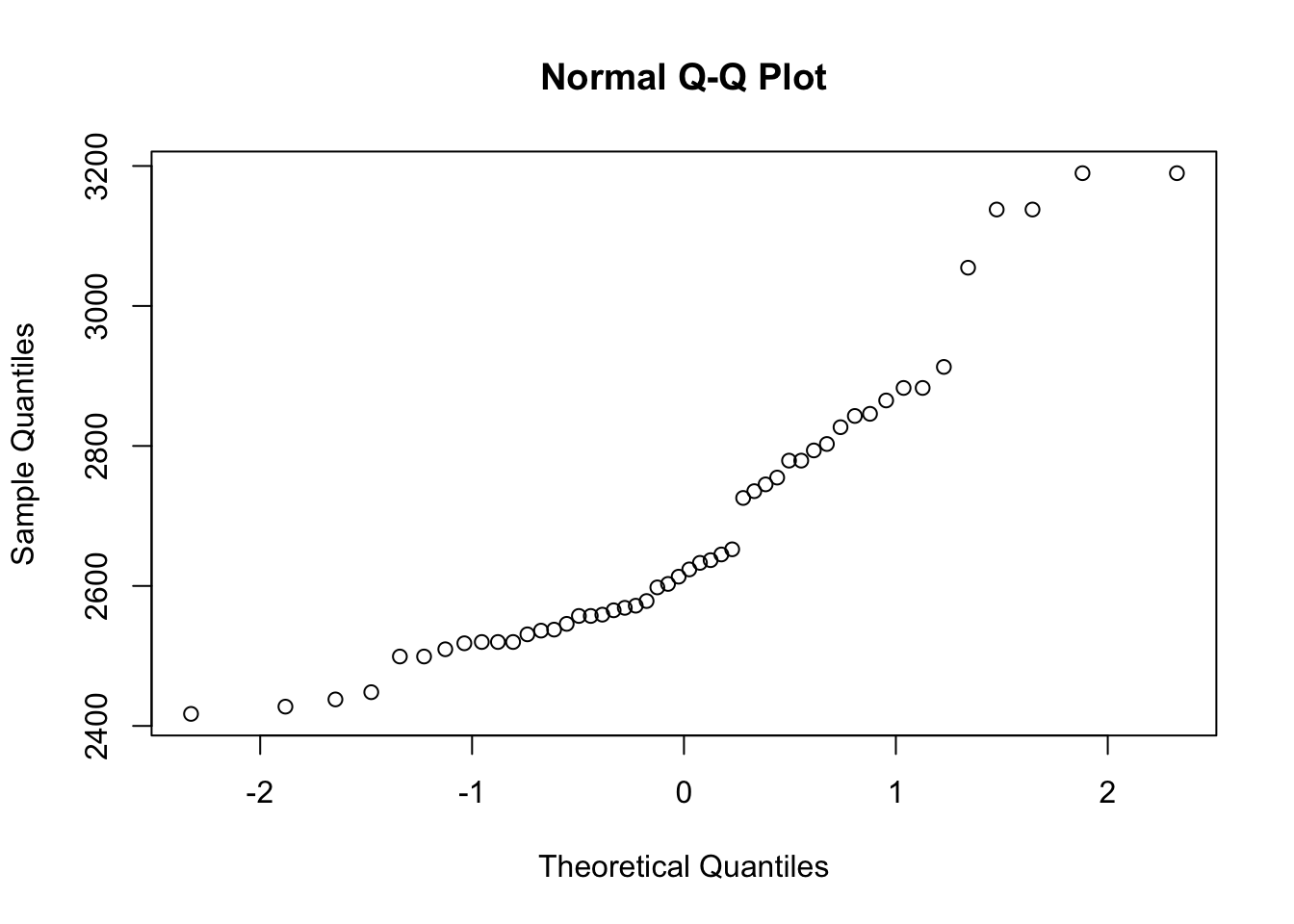
Density and Cumulative Distribution
d <- density(disburse$amount_paid) # density of amount paid

plot(d, main = "Density of Amount Paid")  # plot density

polygon(d, col="violet", border="black") # add color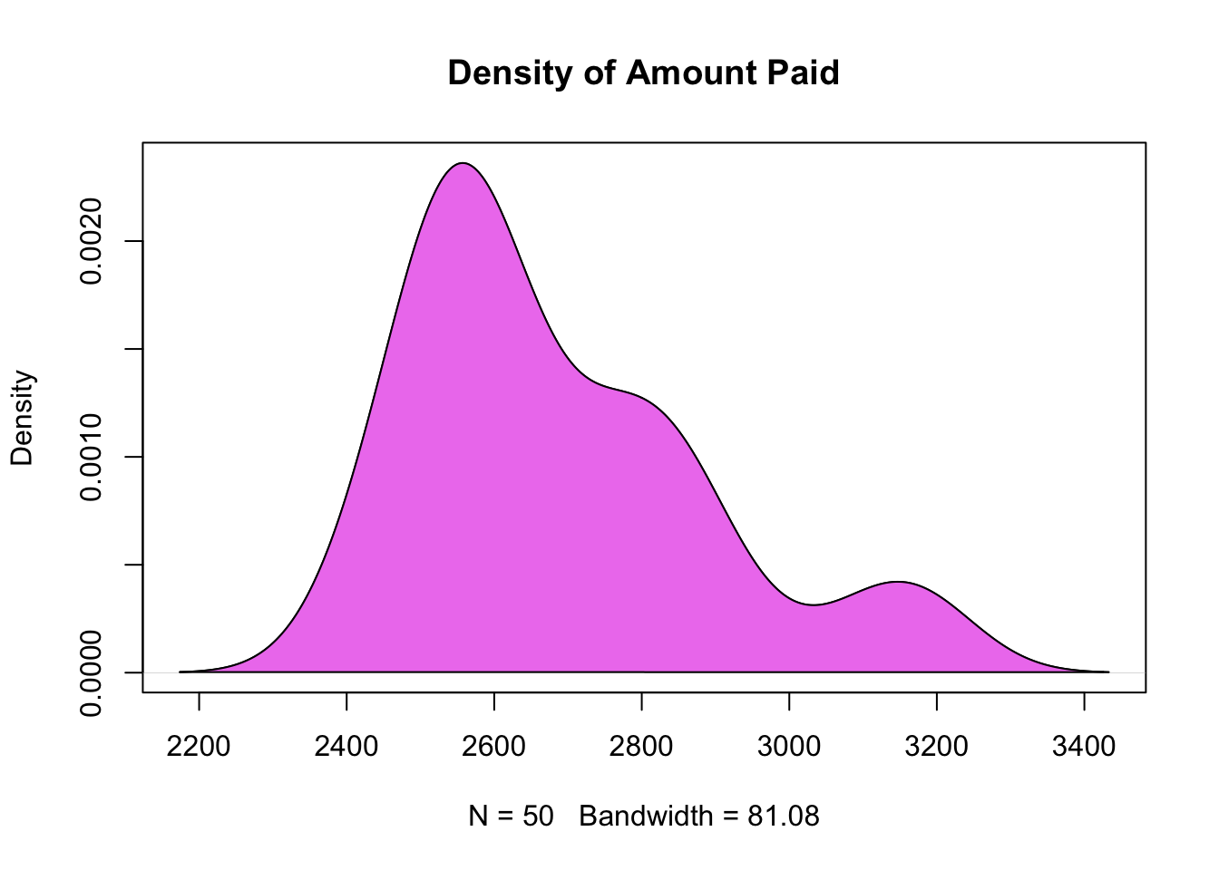
plot(
    ecdf(disburse$amount_paid), # 累積分布関数を計算
    main = "Cumulative Density of Amount Paid" # 図のタイトル
    ) # 誤植 ~いらない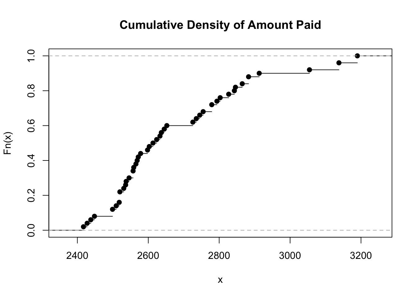
ecdf() is a function that computes the empirical cumulative distribution function of a dataset.
lr <- read_csv(system.file(
"extdata",
"ch_2_data_types.csv",
package = "auditanalytics",
mustWork = TRUE
)
)
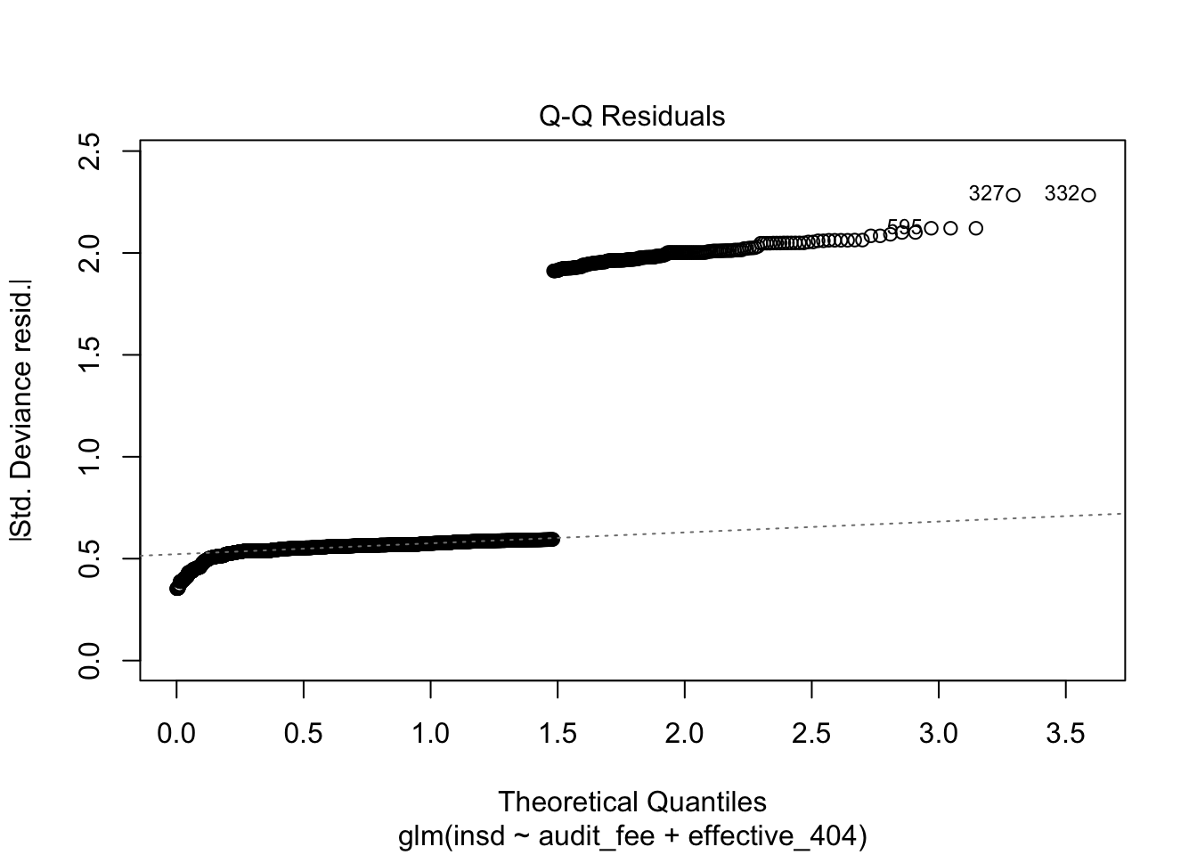
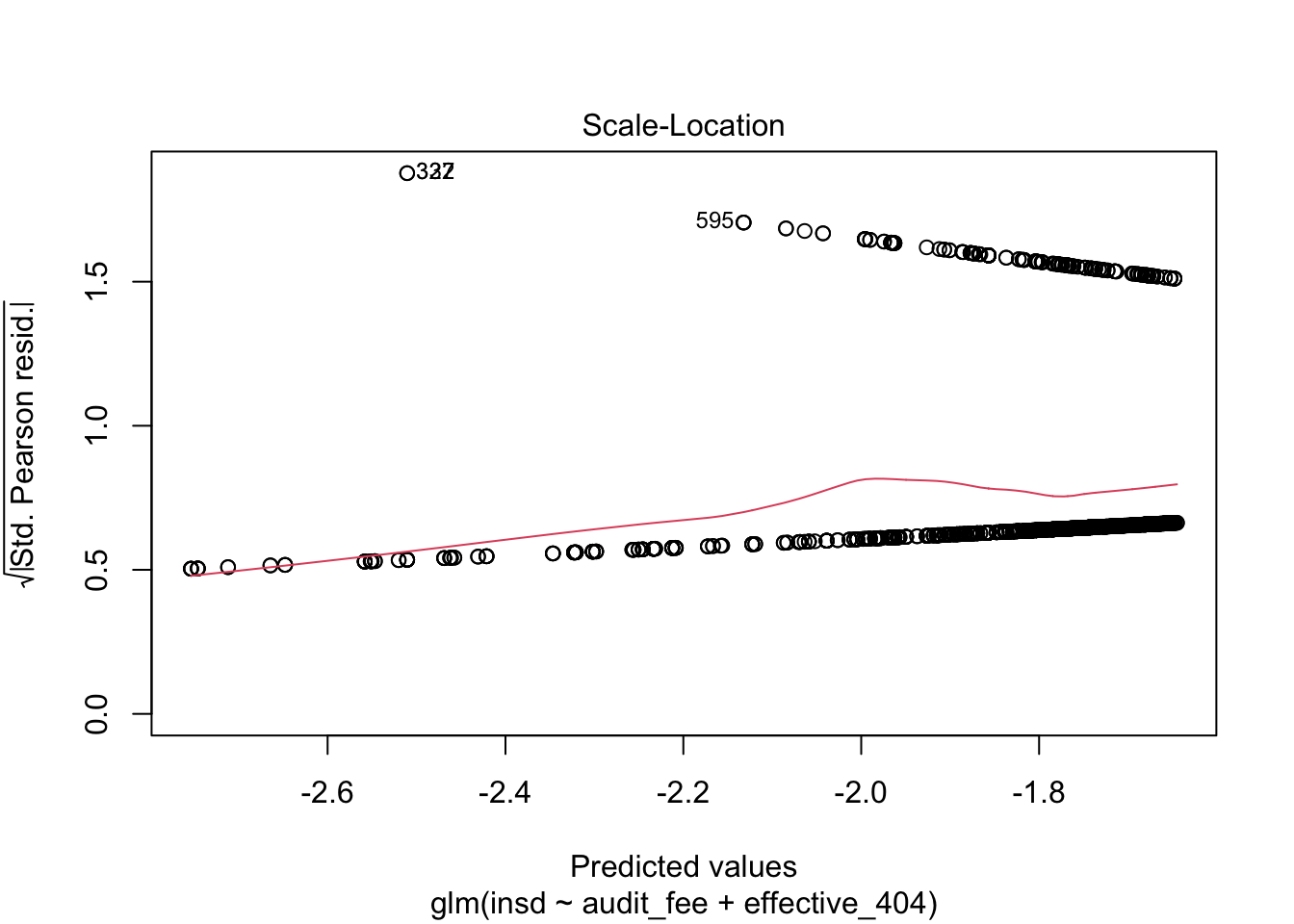
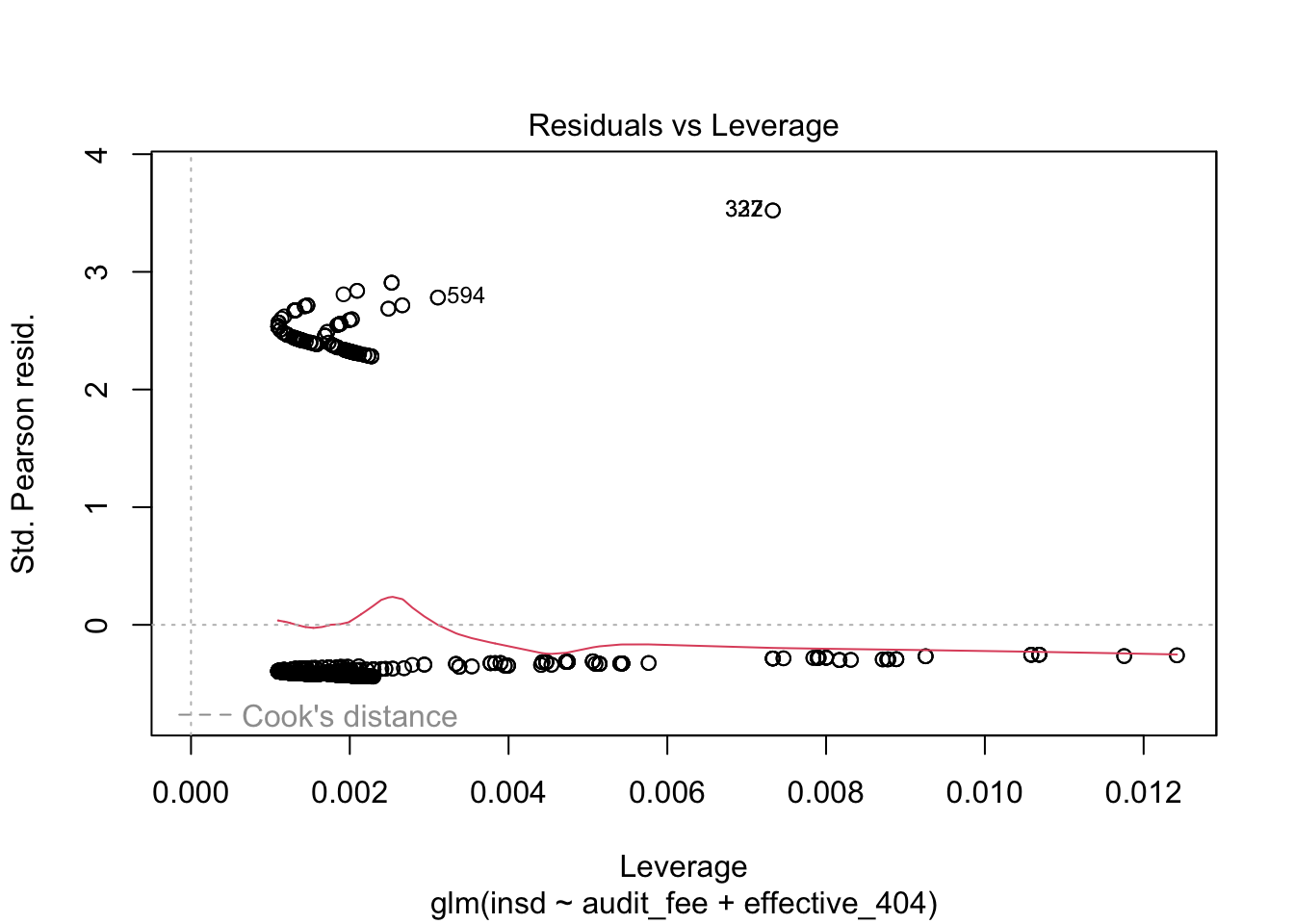
lgt <- glm( # general linear method
formula = insd ~ audit_fee + effective_404, # 回帰モデル
family = "binomial", # link function
data = lr) # data frame
summary(lgt) # 結果の表示
Call:
glm(formula = insd ~ audit_fee + effective_404, family = "binomial",
    data = lr)

Coefficients:
                Estimate Std. Error z value Pr(>|z|)
(Intercept)   -1.732e+00  1.128e-01 -15.354   <2e-16 ***
audit_fee     -9.530e-09  4.496e-09  -2.120    0.034 *
effective_404  8.928e-02  1.518e-01   0.588    0.557
---
Signif. codes:  0 '***' 0.001 '**' 0.01 '*' 0.05 '.' 0.1 ' ' 1

(Dispersion parameter for binomial family taken to be 1)

    Null deviance: 1214.8  on 1511  degrees of freedom
Residual deviance: 1209.4  on 1509  degrees of freedom
  (2 個の観測値が欠損のため削除されました)
AIC: 1215.4

Number of Fisher Scoring iterations: 4plot(lgt) # 図の作成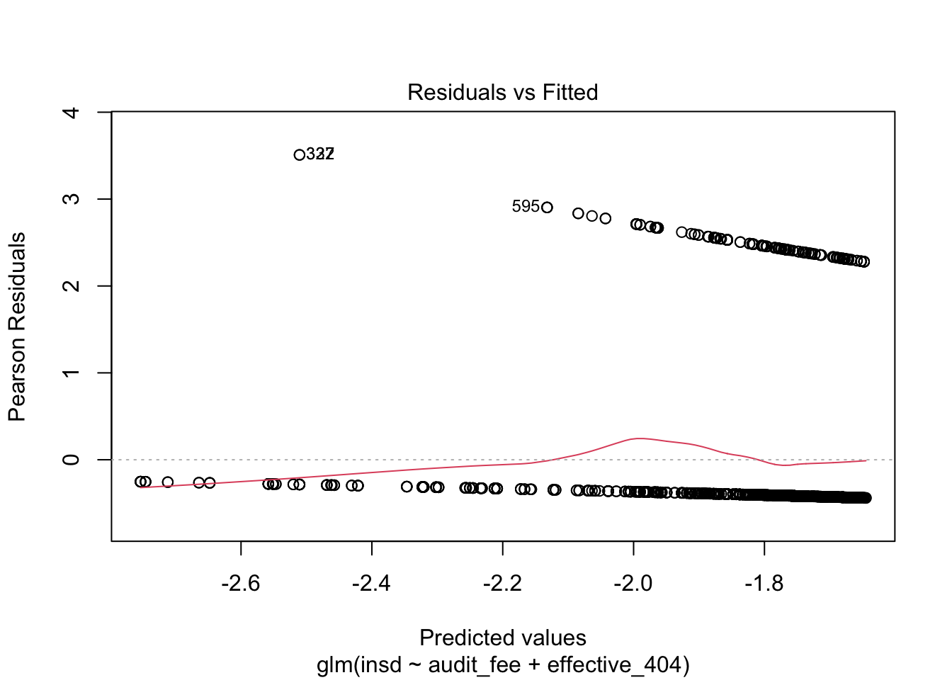
keras
# install.packages("keras") # install keras packages
library(keras)
# install_keras() # Run this only once. Installation takes time.


mnist <- dataset_mnist() # MNISTデータを読み込む

class(mnist)   # List class
[1] "list"glimpse(mnist) # See the structure of the dataList of 2
$ train:List of 2
..$ x: int [1:60000, 1:28, 1:28] 0 0 0 0 0 0 0 0 0 0 ...
..$ y: int [1:60000(1d)] 5 0 4 1 9 2 1 3 1 4 ...
$ test :List of 2
..$ x: int [1:10000, 1:28, 1:28] 0 0 0 0 0 0 0 0 0 0 ...
..$ y: int [1:10000(1d)] 7 2 1 0 4 1 4 9 5 9 ...The MNIST database was constructed from NIST’s Special Database 3 and Special Database 1 which contain binary images of handwritten digits.
train_images <- mnist$train$x # image data for training
train_labels <- mnist$train$y # label data for training
test_images <- mnist$test$x   # test image data
test_labels <- mnist$test$y   # test label data

network <- keras_model_sequential() # null model
network |>
    # 28*28 pixel images are flattened into 784 pixel vectors
    layer_dense(units = 512, input_shape = c(28 * 28)) |>
    # ReLU activation function converts negative values to zero
    layer_activation('relu') |> # ReLU activation function
    layer_dense(units = 10) |>  # 10 output layers 1:10
    # softmax activation function convert the output to a probability distribution
    layer_activation("softmax") # softmax activation function


network |> compile(       # モデルをコンパイル
  optimizer = "rmsprop",  # 最適化アルゴリズム
  loss = "categorical_crossentropy", # 損失関数
  metrics = c("accuracy") # 評価関数
)

# Training data
train_images <- array_reshape( # 行列に変換
    train_images,              # 訓練用画像データ
    c(60000, 28 * 28)          # 画像の形状
    )
# Test data
test_images <- array_reshape( # 行列に変換
    test_images,              # テスト用画像データ
    c(10000, 28 * 28)         # 画像の形状
    )
# 0が黒,255が白のデータを0-1の範囲に正規化
train_images <- train_images / 255
test_images  <- test_images  / 255


train_labels <- to_categorical(train_labels) #
test_labels <- to_categorical(test_labels)   #


history <- network |>
    fit( # training the model
        train_images, # training image data
        train_labels, # training label data
        epochs = 10,  # the number of times the model will be trained
        batch_size = 128 # the number of samples per gradient update
        )
Epoch 1/10
469/469 - 1s - loss: 0.2542 - accuracy: 0.9265 - 1s/epoch - 3ms/step
Epoch 2/10
469/469 - 1s - loss: 0.1031 - accuracy: 0.9696 - 1s/epoch - 3ms/step
Epoch 3/10
469/469 - 1s - loss: 0.0673 - accuracy: 0.9804 - 1s/epoch - 3ms/step
Epoch 4/10
469/469 - 1s - loss: 0.0491 - accuracy: 0.9853 - 1s/epoch - 3ms/step
Epoch 5/10
469/469 - 1s - loss: 0.0370 - accuracy: 0.9893 - 1s/epoch - 3ms/step
Epoch 6/10
469/469 - 1s - loss: 0.0284 - accuracy: 0.9916 - 1s/epoch - 3ms/step
Epoch 7/10
469/469 - 1s - loss: 0.0224 - accuracy: 0.9935 - 1s/epoch - 3ms/step
Epoch 8/10
469/469 - 1s - loss: 0.0167 - accuracy: 0.9952 - 1s/epoch - 3ms/step
Epoch 9/10
469/469 - 1s - loss: 0.0132 - accuracy: 0.9960 - 1s/epoch - 3ms/step
Epoch 10/10
469/469 - 1s - loss: 0.0103 - accuracy: 0.9972 - 1s/epoch - 3ms/stepplot(history) # 訓練の履歴をプロット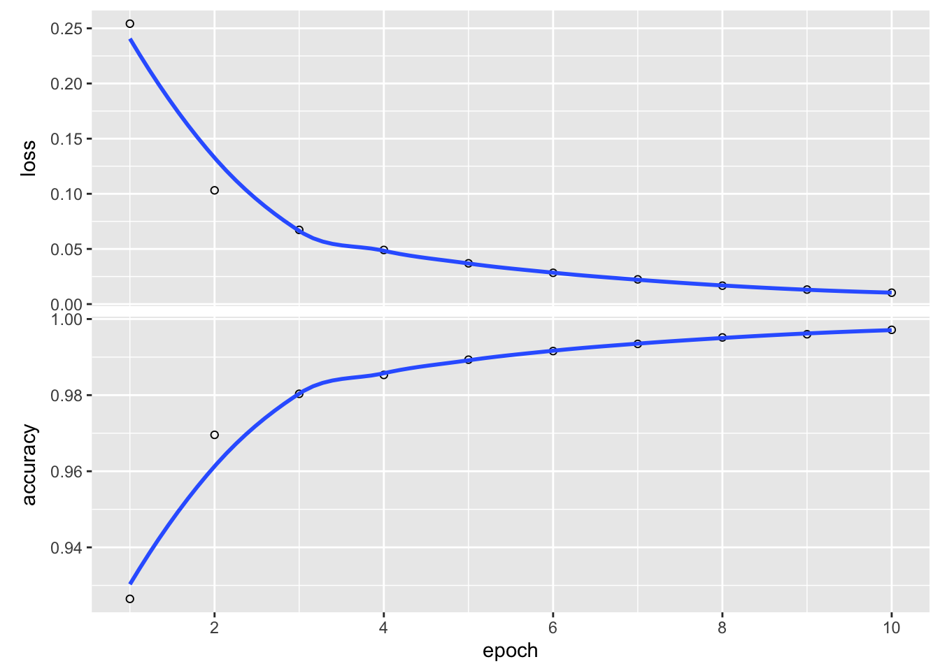
metrics <- network |>
    evaluate(test_images, test_labels, verbose = 0)
metrics |> kable()| x | |
|---|---|
| loss | 0.0665813 |
| accuracy | 0.9820000 |
Chapter 4. Risk Assessment and Audit Planning
Auditing
pacman::p_load(finstr, XBRL, xbrlus, pander, knitr, kableExtra)


old_o <- options(stringsAsFactors = FALSE) # 文字列をファクターとして扱わない

xbrl_data_2016 <- xbrlDoAll("XBRL/gm-20161231.xml")
xbrl_data_2017 <- xbrlDoAll("XBRL/gm-20171231.xml")

options(old_o) # 文字列をファクターとして扱う

st2016 <- xbrl_get_statements(xbrl_data_2016)
st2017 <- xbrl_get_statements(xbrl_data_2017)


print(st2017) # 2017年度の財務諸表
Financial statements repository
From To Rows Columns
ConsolidatedBalanceSheets 2016-12-31 2017-12-31 2 44
ConsolidatedIncomeStatements 2015-12-31 2017-12-31 3 29
ConsolidatedStatementsOfCashFlows 2015-12-31 2017-12-31 3 42
ConsolidatedStatementsOfComprehensiveIncome 2015-12-31 2017-12-31 3 11# 連結貸借対照表を取得
balance_sheet2017 <- st2017$ConsolidatedBalanceSheets
balance_sheet2016 <- st2016$ConsolidatedBalanceSheets
# 連結損益計算書
income2017 <- st2017$ConsolidatedIncomeStatements
income2016 <- st2016$ConsolidatedIncomeStatements
## 貸借対照表を出力
capture.output(
bs_table <- print( # 出力
balance_sheet2017, # オブジェクト名
html = FALSE, # html出力しない
big.mark = ",", # 3桁区切りにカンマを使用
dateFormat = "%Y"), # 日付のフォーマット
file= "NUL") # 出力先をNULにする
bs_table |>
head(10) |> # 先頭10行を表示
kable(
longtable = T, # ページまたぎ
caption = "Balance Sheet", # タイトル
booktabs = T
) |>
kable_styling(
bootstrap_options = c("striped", "hover", "condensed"),
full_width = F,
font_siz = 18
)| Element | 2017-12-31 | 2016-12-31 |
|---|---|---|
| Assets = | 212482 | 221690 |
| + AssetsCurrent = | 68744 | 76203 |
| + CashAndCashEquivalentsAtCarryingValue | 15512 | 12574 |
| + MarketableSecuritiesCurrent | 8313 | 11841 |
| + AccountsNotesAndLoansReceivableNetCurrent | 8164 | 8700 |
| + InventoryNet | 10663 | 11040 |
| + gm_AssetsSubjecttoorAvailableforOperatingLeaseNetCurrent | 1106 | 1110 |
| + OtherAssetsCurrent | 4465 | 3633 |
| + AssetsOfDisposalGroupIncludingDiscontinuedOperationCurrent | 0 | 11178 |
| + NotesAndLoansReceivableNetCurrent | 0 | 0 |
balance_sheet <- balance_sheet2017 |> merge(balance_sheet2016)

capture.output(
    bs_table <- print(
        balance_sheet,
        html = FALSE,
        big.mark = ",",
        dateFormat = "%Y"
        ),
    file = "NUL"
    )

bs_table |>
    head(10) |>
    kable(
        longtable = T,
        caption="Merged Balance Sheet",
        # "latex",
        booktabs = T) |>
    kable_styling(
        bootstrap_options = c("striped", "hover", "condensed"),
        full_width = F,
        font_size = 18
)| Element | 2017-12-31 | 2016-12-31 | 2015-12-31 |
|---|---|---|---|
| Assets = | 212482 | 221690 | 194338 |
| + AssetsCurrent = | 68744 | 76203 | 69408 |
| + CashAndCashEquivalentsAtCarryingValue | 15512 | 12960 | 15238 |
| + MarketableSecuritiesCurrent | 8313 | 11841 | 8163 |
| + AccountsNotesAndLoansReceivableNetCurrent | 8164 | 9638 | 8337 |
| + InventoryNet | 10663 | 13788 | 13764 |
| + gm_AssetsSubjecttoorAvailableforOperatingLeaseNetCurrent | 1106 | 1896 | 2783 |
| + OtherAssetsCurrent | 4465 | 4015 | 3072 |
| + AssetsOfDisposalGroupIncludingDiscontinuedOperationCurrent | 0 | 0 | 0 |
| + NotesAndLoansReceivableNetCurrent | 0 | 0 | 0 |
check <- check_statement(balance_sheet2017)
check
Number of errors: 8
Number of elements in errors: 4
Element: AssetsCurrent = + CashAndCashEquivalentsAtCarryingValue + MarketableSecuritiesCurrent + AccountsNotesAndLoansReceivableNetCurrent + InventoryNet + gm_AssetsSubjecttoorAvailableforOperatingLeaseNetCurrent + OtherAssetsCurrent + AssetsOfDisposalGroupIncludingDiscontinuedOperationCurrent + NotesAndLoansReceivableNetCurrent
date original calculated error
3 2016-12-31 7.6203e+10 6.0076e+10 1.6127e+10
4 2017-12-31 6.8744e+10 4.8223e+10 2.0521e+10
Element: AssetsNoncurrent = + EquityMethodInvestments + PropertyPlantAndEquipmentNet + IntangibleAssetsNetIncludingGoodwill + DeferredIncomeTaxAssetsNet + OtherAssetsNoncurrent + DisposalGroupIncludingDiscontinuedOperationAssetsNoncurrent + NotesAndLoansReceivableNetNoncurrent + PropertySubjectToOrAvailableForOperatingLeaseNet
date original calculated error
5 2016-12-31 1.45487e+11 1.28486e+11 1.7001e+10
6 2017-12-31 1.43738e+11 1.22530e+11 2.1208e+10
Element: LiabilitiesCurrent = + AccountsPayableCurrent + AccruedLiabilitiesCurrent + LiabilitiesOfDisposalGroupIncludingDiscontinuedOperationCurrent + DebtCurrent
date original calculated error
11 2016-12-31 8.5181e+10 6.1384e+10 2.3797e+10
12 2017-12-31 7.6890e+10 4.9925e+10 2.6965e+10
Element: LiabilitiesNoncurrent = + OtherPostretirementDefinedBenefitPlanLiabilitiesNoncurrent + DefinedBenefitPensionPlanLiabilitiesNoncurrent + OtherLiabilitiesNoncurrent + LiabilitiesOfDisposalGroupIncludingDiscontinuedOperationNoncurrent + LongTermDebtAndCapitalLeaseObligations
date original calculated error
13 2016-12-31 9.2434e+10 4.1108e+10 5.1326e+10
14 2017-12-31 9.9392e+10 3.2138e+10 6.7254e+10check_statement(
within(balance_sheet2017, InventoryNet <- InventoryNet * 2)
)Number of errors: 8
Number of elements in errors: 4
Element: AssetsCurrent = + CashAndCashEquivalentsAtCarryingValue + MarketableSecuritiesCurrent + AccountsNotesAndLoansReceivableNetCurrent + InventoryNet + gm_AssetsSubjecttoorAvailableforOperatingLeaseNetCurrent + OtherAssetsCurrent + AssetsOfDisposalGroupIncludingDiscontinuedOperationCurrent + NotesAndLoansReceivableNetCurrent
date original calculated error
3 2016-12-31 7.6203e+10 7.1116e+10 5.087e+09
4 2017-12-31 6.8744e+10 5.8886e+10 9.858e+09
Element: AssetsNoncurrent = + EquityMethodInvestments + PropertyPlantAndEquipmentNet + IntangibleAssetsNetIncludingGoodwill + DeferredIncomeTaxAssetsNet + OtherAssetsNoncurrent + DisposalGroupIncludingDiscontinuedOperationAssetsNoncurrent + NotesAndLoansReceivableNetNoncurrent + PropertySubjectToOrAvailableForOperatingLeaseNet
date original calculated error
5 2016-12-31 1.45487e+11 1.28486e+11 1.7001e+10
6 2017-12-31 1.43738e+11 1.22530e+11 2.1208e+10
Element: LiabilitiesCurrent = + AccountsPayableCurrent + AccruedLiabilitiesCurrent + LiabilitiesOfDisposalGroupIncludingDiscontinuedOperationCurrent + DebtCurrent
date original calculated error
11 2016-12-31 8.5181e+10 6.1384e+10 2.3797e+10
12 2017-12-31 7.6890e+10 4.9925e+10 2.6965e+10
Element: LiabilitiesNoncurrent = + OtherPostretirementDefinedBenefitPlanLiabilitiesNoncurrent + DefinedBenefitPensionPlanLiabilitiesNoncurrent + OtherLiabilitiesNoncurrent + LiabilitiesOfDisposalGroupIncludingDiscontinuedOperationNoncurrent + LongTermDebtAndCapitalLeaseObligations
date original calculated error
13 2016-12-31 9.2434e+10 4.1108e+10 5.1326e+10
14 2017-12-31 9.9392e+10 3.2138e+10 6.7254e+10check <- check_statement(income2017, element_id = "OperatingIncomeLoss")
checkNumber of errors: 0
Number of elements in errors: 0 check$expression[1][1] "+ Revenues - CostsAndExpenses"check$calculated / 10^6[1] 5538 9962 10016Rearranging the Statement
expose() function
expose(balance_sheet,
    # Assets
    "Current Assets" = "AssetsCurrent",
    "Noncurrent Assets" = other("Assets"),
    # Liabilites and equity
    "Current Liabilities" = "LiabilitiesCurrent",
    "Noncurrent Liabilities" = other(c("Liabilities", "CommitmentsAndContingencies")),
    "Stockholders Equity" = "StockholdersEquity"
)
Financial statement: 3 observations from 2015-12-31 to 2017-12-31
Element 2017-12-31 2016-12-31 2015-12-31
Assets = 212482 221690 194338
+ Current.Assets 48223 54138 51357
+ Noncurrent.Assets 122530 90237 86258
LiabilitiesAndStockholdersEquity = 212482 221690 194338
+ Current.Liabilities 49925 56153 51655
+ Noncurrent.Liabilities 32138 36834 39249
+ Stockholders.Equity 35001 43836 39871
+ OtherLiabilitiesAndStockholdersEquity_ 1199 239 452 expose(balance_sheet,
# Assets
"Tangible Assets" = "Assets" %without% c(
"AssetsOfDisposalGroupIncludingDiscontinuedOperationCurrent",
"NotesAndLoansReceivableNetCurrent",
"gm_AssetsSubjecttoorAvailableforOperatingLeaseNetCurrent"
),
"Intangible Assets" = other("Assets"),
# Liabilites and equity
"Liabilities" = c("Liabilities", "CommitmentsAndContingencies"),
"Stockholders Equity" = "StockholdersEquity"
)Financial statement: 3 observations from 2015-12-31 to 2017-12-31
Element 2017-12-31 2016-12-31 2015-12-31
Assets = 212482 221690 194338
+ Tangible.Assets 169647 142479 134832
+ Intangible.Assets 1106 1896 2783
LiabilitiesAndStockholdersEquity = 212482 221690 194338
+ Liabilities 82063 92987 90904
+ Stockholders.Equity 35001 43836 39871
+ OtherLiabilitiesAndStockholdersEquity_ 1199 239 452 diff_bs <- diff(balance_sheet)
capture.output(
bs_table <- print(
diff_bs,
html = FALSE,
big.mark = ",",
dateFormat = "%Y"
), file = "NUL")
bs_table |>
head(10) |>
kable(longtable = T,
caption = "Lagged Differences in Balance Sheets",
# "latex",
booktabs = T) |>
kable_styling(
bootstrap_options = c("striped", "hover", "condensed"),
full_width = F,
font_size = 18)| Element | 2017-12-31 | 2016-12-31 |
|---|---|---|
| Assets = | -9208 | 27352 |
| + AssetsCurrent = | -7459 | 6795 |
| + CashAndCashEquivalentsAtCarryingValue | 2552 | -2278 |
| + MarketableSecuritiesCurrent | -3528 | 3678 |
| + AccountsNotesAndLoansReceivableNetCurrent | -1474 | 1301 |
| + InventoryNet | -3125 | 24 |
| + gm_AssetsSubjecttoorAvailableforOperatingLeaseNetCurrent | -790 | -887 |
| + OtherAssetsCurrent | 450 | 943 |
| + AssetsOfDisposalGroupIncludingDiscontinuedOperationCurrent | 0 | 0 |
| + NotesAndLoansReceivableNetCurrent | 0 | 0 |
pacman::p_load(finreportr)

tesla_ann <- AnnualReports("TSLA")
tesla_ann
tesla_inc <- GetIncome("TSLA", 2018)
tesla_bs <- GetBalanceSheet("TSLA", 2018)
tesla_cf <- GetCashFlow("TSLA", 2018)
head(tesla_inc)
But this code will not be able to access Tesla’s 2019 reports, because it throws an error:
edgar package
pacman::p_load(xml2, curl, edgar)
u1 <- "https://www.sec.gov/Archives/edgar/data/1318605/000156459020004475/tsla-10k_20191231_htm.xml"
url_file <- curl_download(u1, destfile = "~/Downloads/u1.xml") # to download and save
list_url_1 <- as_list(read_xml(u1)) # to read into R

cik.no <- 0001318605 # Tesla
form.type <- "10-K"
filing.year = 2019
quarter = c(1,2,3,4)

getFilings(
    cik.no,
    form.type,
    filing.year,
    quarter,
    downl.permit = "y"
)NULLになりました。
Audit Staffing and Budgets
Audit Staffing and Budgets
benefit <- seq(10, 10000, 10) # 10から10000まで10刻み
staff_allocated <- data.frame(benefit, floor(10 * (log(benefit^.06))))

ggplot(staff_allocated, aes(staff_allocated[,1],staff_allocated[,2]) ) +
    geom_line() + labs(x ="Audit Risk Reduction",  y ="Staff Auditor Person-Months")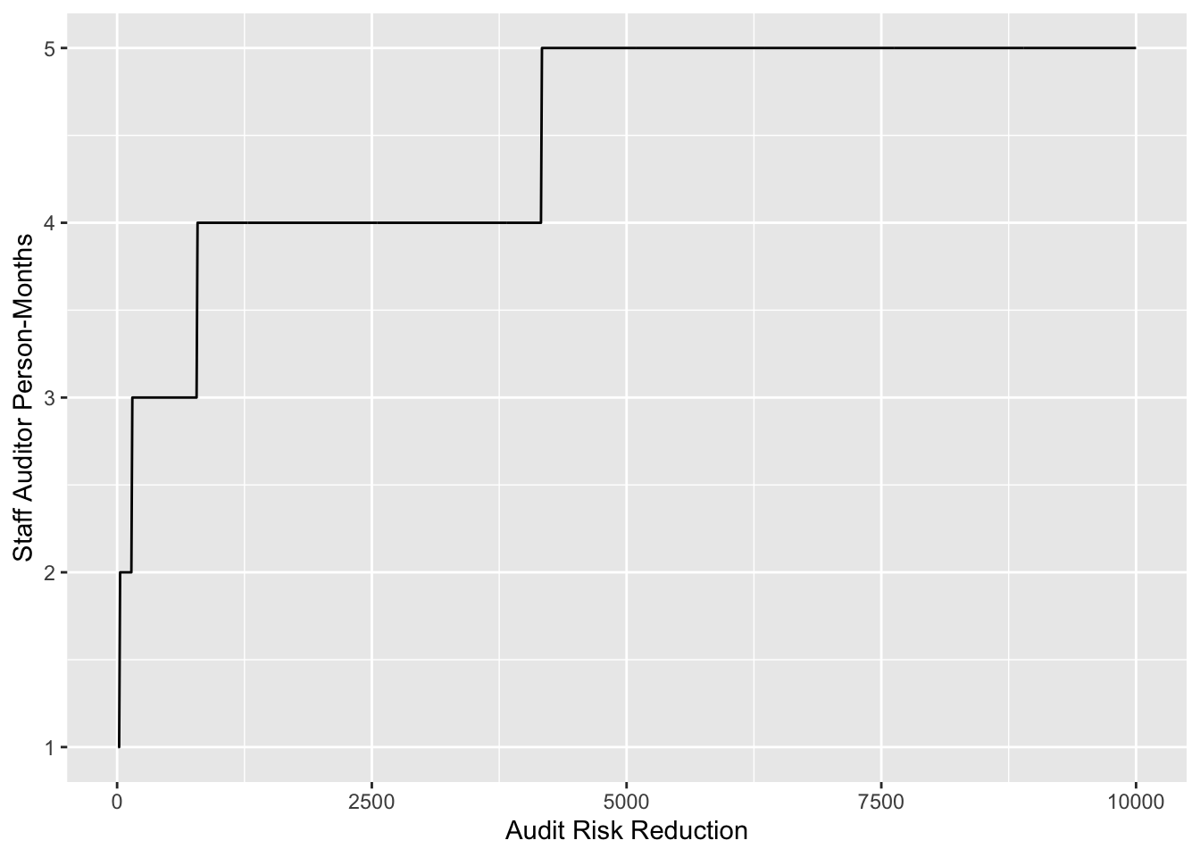
Shiny App
# Define UI for application
library(shiny) # Load the shiny package

ui <- fluidPage(
    titlePanel("Risk Assessment Matrix"),
    sidebarLayout(
        sidebarPanel(
            # Input: 監査テストの統計的信頼水準
            sliderInput("confidence", "Confidence:",
                        min = .7,
                        max = .999,
                        value = .95),
            # Input: サンプル取引ごとの監査コスト
            sliderInput("cost", "Audit $ / transaction:",
                        min = 0,
                        max = 500,
                        value = 100),
            # Input: Text for providing a caption for the RAM
            textInput(
                inputId = "caption",
                label = "クライアント:",
                value = "XYZ Corp.")
        ),
        # Main panel for displaying outputs
        mainPanel(
            # Output: slider values entered
            tableOutput("values"),
            # Output: Formatted text for caption
            h3(textOutput("caption", container = span)),
            # Output: total cost of the audit
            textOutput("view"),
            # Output: RAM summary with sample sizes (scope) and cost
            verbatimTextOutput("summary"),
            h6("リスク選択: 1 = 低, 2 = 中, 3 = 高"),
            h6("リスク知能 = ビジネス・インテリジェンス・スキャンニングで示されるリスク水準"),
            h6("前年度リスク = 前期に監査人が示したリスク水準"),
            h6("Scope = estimated discovery sample size that will be needed in the audit of this account"),
            h6("Audit cost = audit labor dollars per sampled transaction"),
            h6("Confidence = statistical confidence"),
            h6("Account Amount and the Ave. Transaction size are in $ without decimals or 000 dividers")
        )
    )
)

# サーバー側の設定
server <- function(input, output) {
    ram <- read.csv(system.file("extdata",
        "risk_asst_matrix.csv",
        package = "auditanalytics",
        mustWork = TRUE)
        )

    sliderValues <- reactive({
        data.frame(
            Audit_Parameter = c("confidence", "cost"),
            Value = as.character(c(input$confidence, input$cost)),
            stringsAsFactors = FALSE)
        })

    output$values <- renderTable({
        sliderValues()
        })

    output$caption <- renderText({
        input$caption
        })

    output$summary <- renderPrint({
        ram <- ram
        conf <- input$confidence
        cost <- input$cost
        risk <- (10 - (as.numeric(ram[,2]) * as.numeric(ram[,3])) )/100
        Scope <-  ceiling( log(1-conf) / log( 1- risk))
        ram <- cbind(ram[,1:5], Scope)
        Min_cost <- Scope * cost
        ram <- cbind(ram[,1:6], Min_cost)
        ram
        })

    output$view <- renderText({ # 監査費用を表示
        ram <- ram # リスク評価行列を読み込む
        conf <- input$confidence # 監査の信頼度
        cost <- input$cost # 監査費用
        risk <- (10 - (as.numeric(ram[,2]) * as.numeric(ram[,3])) )/100 # リスク
        Scope <-  ceiling( log(1-conf) / log( 1- risk)) # 範囲
        ram <- cbind(ram[,1:5], Scope) # リスク評価行列に範囲を追加
        Min_cost <- Scope * cost # 最小監査費用を計算
        minimum_audit_cost <- sum(Min_cost) # 最小監査費用を合計
        c("Minimum estimated audit cost = ",minimum_audit_cost) # 最小監査費用を表示
        })
}
# Run the application
shinyApp(ui = ui, server = server)Generating the Audit Budget from the Risk Assessment Matrix
confidence <- seq(.99, 0.7, -0.01) # 0.99から0.7まで0.01刻みのベクトル
n <- (log(1 - confidence)) / log(1 - 0.05) # 発見サンプルサイズを計算
plot(confidence,n, type="l") # 発見サンプルサイズをプロット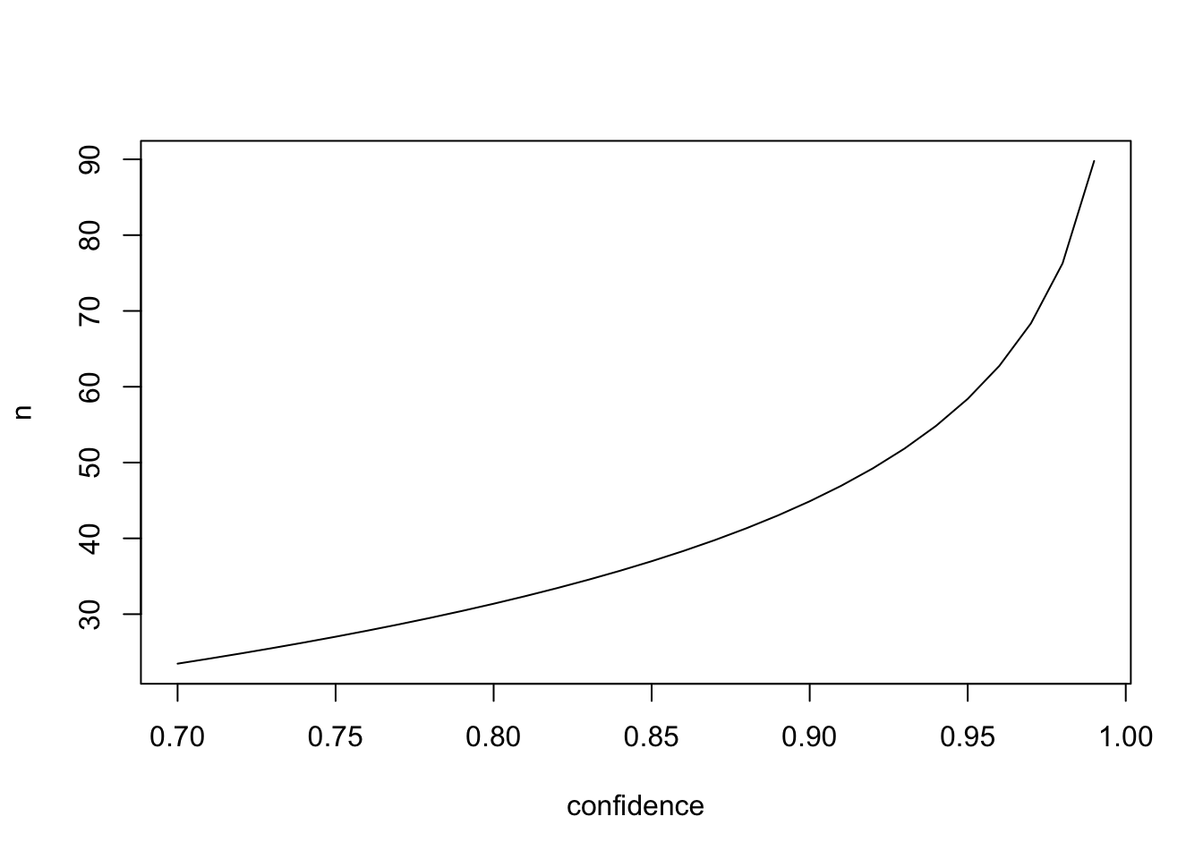
confidence <- 0.95
n <- (log(1 - confidence)) / log(1 - 0.05)
cat("\n Discovery sample size = ", ceiling(n))
Discovery sample size = 59# install.packages("pwr") # first time only
library(pwr) # Cohen本のpower analysis
size <- 1000 # トランザクションの総数
Delta <- 0.05 * size # 5%の許容エラー率を検出する
sigma <- 0.3 * size # 変動(おそらく1/3)を推測する
effect <- Delta/sigma # 許容度÷変動
sample <- pwr.t.test( # pwr.t.test関数を使用
d = effect, sig.level = 0.05, power = 0.8,
type = "one.sample",
alternative = "greater" ## look for overstatement of earnings
)
cat("\n Attribute sample size for occurrence of error = ", ceiling(sample$n))
Attribute sample size for occurrence of error = 224size: 総トランザクション数(ここでは1000)。Delta: 許容エラー率として5%を想定しており、1000件中5%である「50件のエラーを検出できるようにしたい」という設定。sigma: 変動の範囲としてトランザクション数の約30%(1/3)を想定し、標準偏差に相当effect: 効果の大きさ(エラー率÷変動)で、これが実際に検出したい差を標準化したものd = effect: effectで計算された効果の大きさを指定。これは検出したいエラー率が、変動に対してどれだけの比率かを示しています。- sig.level = 0.05: 有意水準を5%に設定。
power = 0.8: 検出力(power)を80%に設定。これは、実際に効果が存在する場合にそれを80%の確率で検出できることを意味します。type = "one.sample": 1標本のt検定を使用する設定。つまり、1つの標本の平均が期待値と異なるかどうかを調べるもの。alternative = "greater": 片側検定で、「平均が期待よりも大きい」場合(例:利益の過大計上)を検出したいことを示しています。
size   <- 100000      # 取引の総額
mu     <- 50          # 取引の平均値
Delta  <- 0.05 * mu   # 5%の金額の許容誤差を検出
sigma  <- 30          # 変動
effect <- Delta / sigma # 許容度÷変動

sample <- pwr.t.test( # Cohenのpower analysis
  d = effect,       # Cohenのd
  sig.level = 0.05, # 有意水準
  power = 0.8,      # 効果量
  type = "one.sample", # 一標本検定
  alternative = "greater" # 偽陽性
  )
cat("\n Attribute sample size for amount of error = ", ceiling(sample$n))
Attribute sample size for amount of error = 892