外国書購読 Day4
Risk Assessment and Planning

Soichi Matsuura

2024-10-23

Machine Learning Methods

• Over the past decade, very useful extensions to twentieth century statistical models have been provided by advances in machine learning, and in particular deep-learning.
• Inference is a decision \delta (estimation, prediction) based on data x \in X that hopefully contains information about a particular set of constructs.
• Inference may be about:
  1. Classification — e.g., identifying faces, threats.
  2. Estimation — e.g., a vector \theta = \{\theta_1, \dots , \theta_n\}.
  3. Other decisions that may or may not be carried out in real time; e.g., driving a car.

Goals of Machine Learning

• The implicit goal of machine learning is construction of decision strategies that minimize risk.
• Risk is an informal concept inherited from gambling, and roughly implies the expected loss from using a given decision strategy \delta.
• Frequentist and Bayesian statisticians both base their decision strategies on real-world data, but sharply divided on the actual implementation and interpretation of decision risk.

Risk and AI

• In practice, risk presents deep learning (and AI in general) with its greatest challenges.
• For example, self-driving cars are trained on massive datasets extracted from many other cars; that knowledge of how to drive is encapsulated in weights in a network model that is firm-wired into a computer unit in a car.
• It matters whether that unit was trained to save pedestrians, or to save property, or to save the driver - each implies a different decision risk.

• Traditionally, statistics have used a squared-error loss function l(\theta, \delta (X)) = \mathrm{E}_{\delta} [\delta (X) - \theta )^2] where \delta(X) = \hat{\theta} in the case of estimation.
• But most real-world decisions are not optimally made with squared-error loss functions.
• Although squared-error loss is still widely used, machine learning practitioners will also use more complex, sometimes asymmetric loss functions that more closely fit the real-world problems.
• Business situations prefer asymmetric loss that penalizes costs and rewards revenues.

Search Algorithms

• Whereas traditional statistics relies heavily on first-order conditions from calculus, deep learning uses compute-intensive search algorithms that explore the response surface of the risk function.
• The following example presents the “Hello World” of machine learning: recognizing handwritten numbers on the National Institute of Standards dataset.

keras

Examples below assume that Tensorflow is installed. See https://www.tensorflow.org/install/。

# install.packages("keras") # install keras packages
pacman::p_load(keras, tidyverse, knitr, kableExtra)
# install_keras() # Run this only once. Installation takes time.

mnist <- dataset_mnist() # MNISTデータを読み込む
class(mnist)   # List class

[1] "list"

glimpse(mnist) # See the structure of the data

List of 2
 $ train:List of 2
  ..$ x: int [1:60000, 1:28, 1:28] 0 0 0 0 0 0 0 0 0 0 ...
  ..$ y: int [1:60000(1d)] 5 0 4 1 9 2 1 3 1 4 ...
 $ test :List of 2
  ..$ x: int [1:10000, 1:28, 1:28] 0 0 0 0 0 0 0 0 0 0 ...
  ..$ y: int [1:10000(1d)] 7 2 1 0 4 1 4 9 5 9 ...

The MNIST database was constructed from NIST’s Special Database 3 and Special Database 1 which contain binary images of handwritten digits.

train_images <- mnist$train$x # image data for training
train_labels <- mnist$train$y # label data for training
test_images <- mnist$test$x   # test image data
test_labels <- mnist$test$y   # test label data

Construct a neural network model. Keras Model composed of a linear stack of layers.

network <- keras_model_sequential() # null model
network |>
    # 28*28 pixel images are flattened into 784 pixel vectors
    layer_dense(units = 512, input_shape = c(28 * 28)) |>
    # ReLU activation function converts negative values to zero
    layer_activation('relu') |> # ReLU activation function
    layer_dense(units = 10) |>  # 10 output layers 1:10
    # softmax activation function convert the output to a probability distribution
    layer_activation("softmax") # softmax activation function

Specify the algorithm and function series.

network |> compile(       # モデルをコンパイル
  optimizer = "rmsprop",  # 最適化アルゴリズム
  loss = "categorical_crossentropy", # 損失関数
  metrics = c("accuracy") # 評価関数
)

Training and Test Data

# Training data
train_images <- array_reshape( # 行列に変換
    train_images,              # 訓練用画像データ
    c(60000, 28 * 28)          # 画像の形状
    )
# Test data
test_images <- array_reshape( # 行列に変換
    test_images,              # テスト用画像データ
    c(10000, 28 * 28)         # 画像の形状
    )
# 0が黒，255が白のデータを0-1の範囲に正規化
train_images <- train_images / 255
test_images  <- test_images  / 255

train_labels <- to_categorical(train_labels) #
test_labels <- to_categorical(test_labels)   #

• Label data is one hot encoded.

• to_categolical() takes a vector or 1 column matrix of class labels and converts it into a matrix with p columns, one for each category.

• (補足) 0〜9の手書き文字の大小関係は今回関係ないため，10個のカテゴリーを意味する10列の行列に変換してます。

Training the Model

history <- network |>
    fit( # training the model
        train_images, # training image data
        train_labels, # training label data
        epochs = 10,  # the number of times the model will be trained
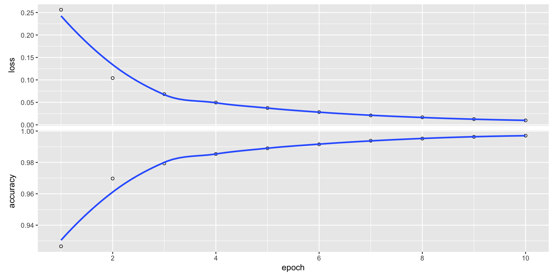
        batch_size = 128) # the number of samples per gradient update

Epoch 1/10
469/469 - 1s - loss: 0.2562 - accuracy: 0.9265 - 1s/epoch - 2ms/step
Epoch 2/10
469/469 - 1s - loss: 0.1040 - accuracy: 0.9697 - 799ms/epoch - 2ms/step
Epoch 3/10
469/469 - 1s - loss: 0.0683 - accuracy: 0.9794 - 795ms/epoch - 2ms/step
Epoch 4/10
469/469 - 1s - loss: 0.0496 - accuracy: 0.9854 - 789ms/epoch - 2ms/step
Epoch 5/10
469/469 - 1s - loss: 0.0375 - accuracy: 0.9890 - 792ms/epoch - 2ms/step
Epoch 6/10
469/469 - 1s - loss: 0.0283 - accuracy: 0.9915 - 795ms/epoch - 2ms/step
Epoch 7/10
469/469 - 1s - loss: 0.0210 - accuracy: 0.9938 - 787ms/epoch - 2ms/step
Epoch 8/10
469/469 - 1s - loss: 0.0168 - accuracy: 0.9952 - 785ms/epoch - 2ms/step
Epoch 9/10
469/469 - 1s - loss: 0.0127 - accuracy: 0.9963 - 783ms/epoch - 2ms/step
Epoch 10/10
469/469 - 1s - loss: 0.0098 - accuracy: 0.9970 - 784ms/epoch - 2ms/step

Plot

plot(history) # 訓練の履歴をプロット

model evaluation

metrics <- network |>
    evaluate(test_images, test_labels, verbose = 0)
metrics |> kable()

	x
loss	0.0736921
accuracy	0.9807000

keras model

• This particular Keras model overfits the MNIST data, with a final accuracy of 98% and loss of 7%.

• Machine learning is a vast and rapidly evolving field.

• It is increasingly for the analysis of social network and other text based intelligence required for the analytical review portion (and other parts) of the audit.

• In the future, expect its role in auditing to expand, as suitable models are developed in the field.

Statistical Perspectives on Audit Evidence and its Information Content

補足

パラメータが\thetaである母集団の従う分布の確率密度関数をf(x \mid \theta)とする。 そのとき，尤度関数と対数尤度関数は、

L (\theta) = f(x \mid \theta), \quad l (\theta) = \log L(\theta)

となり，スコア関数は次式で定義される。

\frac{\partial}{\partial \theta} \log l (\theta)

Support and the Additivity of Evidence: The Log-Likelihood

• The log-likelihood has an intuitive interpretation, as suggested by the term “support.”
• Given independent events, the overall log-likelihood is the sum of the log-likelihoods of the individual events, just as the overall log-probability is the sum of the log-probability of the individual events.
• Viewing data as evidence, this is interpreted as “support from independent evidence adds,” and the log-likelihood is the “weight of evidence.”

The “Score”　

• In statistics, the score (or informant) is the gradient of the log-likelihood function with respect to the parameter vector.
• Evaluated at a particular point, the score indicates the steepness of the log-likelihood function and thereby the sensitivity to infinitesimal changes to the parameter values.
• Since the score is a function of the observations that are subject to sampling error, it lends itself to a test statistic known as score test in which the parameter is held at a particular value.

Fisher Information

• In mathematical statistics, the Fisher information is a way of measuring the amount of information that an observable random variable X carries about an unknown parameter \theta of a distribution that models X.
• Formally, it is the variance of the score, or the expected value of the observed information.
• The Fisher information is a way of measuring the amount of information that an observable random variable X carries about an unknown parameter \theta upon which the probability of X depends.

Risk Assessment and Audit Planning

Auditing

Auditing

• Auditing of financial accounts is the process of verifying that economic events in the real world are accurately summarized in the financial statements of a legal entity.
• An audit opinion, the product of such auditing provides:
  1. Reasonable assurance.
  2. By an independent third party.
  3. Financial statements are presented fairly in all material respects.
  4. In accordance to some financial reporting framework, e.g., GAAP.
  5. Applied consistently so that year-to-year trends and comparisons are possible.

財務諸表監査は、現実世界における経済事象が事業体の財務諸表に正確に記載されているかどうかを検証するプロセスである。 このような監査の成果である監査意見は、下記の点について独立した第三者による合理的保証を提供するものである。 1. 合理的保証。 2. 独立した第三者による。 3. 財務諸表がすべての重要な点において適正に表示されていること。 4. ある財務報告の枠組み（たとえばGAAP）に準拠していること。 5. 継続性をもって適用されているため、年度間の傾向と比較が可能であること。

• In the USA, the auditing framework is dictated by generally accepted accounting principles (GAAP) and generally accepted auditing standards (GAAS).
• Internationally the International Standards on Auditing (ISA) issued by the International Auditing and Assurance Standards Board (IAASB) is considered as the benchmark for audit process.
• Under US generally accepted accounting principles (GAAP) auditors must release one of three types of opinions of the overall financial statements:

1. An unqualified auditor’s opinion is the opinion that the financial statements are presented fairly.
2. A qualified opinion is that the financial statements are presented fairly in all material respects in accordance with GAAP:
   1. Except for a material misstatement that does not pervasively affect the users ability to rely on the financial statements.
   2. Or with a scope limitation that is of limited significance.
3. An adverse audit opinion is issued when the financial statements do not present fairly due to departure from US GAAP with an explanation of the nature and size of the misstatement.

1. 無限定適正意見（unqualified opinion）は、財務諸表が適正に表示されているという意見である。
2. 限定付適正意見（qualified opinion）は、財務諸表がすべての重要な点においてGAAPに準拠して適正に表示されていると認められるものの、下記のような意見の限定と範囲の限定がある。
   1. 財務諸表を信頼する利用者の判断に広範な影響を与えない重要な虚偽表示が存在する。
   2. 重要であるが広範ではない監査範囲の限定が存在する。
3. GAAPに準拠しないことにより財務諸表が適正に表示されていない場合には、監査意見として不適正意見（adverse opinion）が表明される。不適正意見には、虚偽表示の種類と影響についての説明が記載される。

• Additionally an auditor can issue a disclaimer which is considered a type of qualified opinion because there is insufficient and appropriate evidence to form an opinion or because of lack of independence.

1. Unqualified (Clean) Opinion : We believe these financial statements are (1) fairly presented in (2) accordance with GAAP (3) consistently applied.
2. Qualified Opinion : We believe these financial statements are (1) fairly presented in (2) accordance with GAAP (3) consistently applied; except for (4) A List of Exceptions.
3. Adverse Opinion: We DO NOT believe these financial statements are (1) fairly presented in (2) accordance with GAAP (3) consistently applied; THE AUDITORS DISAGREE WITH A List of Exceptions.

1. 無限定適正意見： 監査人は、これらの財務諸表が（1）継続的に適用された（2）GAAPに準拠して（2）適正に表示されていると判断している。
2. 条件付適正意見：監査人は、これらの財務諸表が（1）除外事項を除いて、（2）継続的に適用された（3）GAAPに準拠して（4）適正に表示されていると判断している。
3. 反対意見：監査人は、これらの財務諸表が（1）継続的に適用された（2）GAAPに準拠して（2）適正に表示されていると判断していない。

Risk Assessment in Audit Planning

Risk Assessment

• Risk assessment in auditing is the determination of quantitative value of risk of a particular subset of accounting operations related to the rendering of the audit opinion - i.e., on whether the accounts have material error when GAAP has been consistently applied.
• Quantitative risk assessment requires calculations of two components of risk — the magnitude of the potential loss, and the probability that the loss will occur.
• An accounting cycle begins when accounting personnel create a transaction from a source document and ends with the completion of the financial reports and closing of temporary accounts in preparation for a new cycle.

5 Accounting Cycles

The five accounting cycles are: 1. Revenue cycle. 2. Expenditure cycle (this cycle focuses on two separate resources: inventory and human resources and often considers two separate cycles: purchasing and payroll/HR ). 3. Conversion cycle (Production cycle). 4. Financing (Capital Acquisition and repayment). 5. Fixed assets.

• Problems in any transaction generated in these cycles are the sources of “loss” considered in the Risk Assessment Matrix (RAM).

• Risk assessment consists of subjective and objective evaluations of risk in which assumptions and uncertainties are clearly considered and presented.

• Part of the difficulty in risk management is that measurement of both potential loss and probability of occurrence is error prone and subjective.

• Risk with a large potential loss and a low probability of occurring is often treated differently from one with a low potential loss and a high likelihood of occurring.

• In theory, both are of nearly equal priority, but in practice it can be very difficult to manage when faced with the scarcity of resources, especially time, in which to conduct the risk management process.
• This is one conundrum engendered by auditing’s inherently “wicked” character.
• A Risk Assessment Matrix (RAM) is a calculation spreadsheet that is used in risk assessment to define, estimate, argue, and support particular risks involved in decision-making.
• In auditing, the objective of the RAM is to construct a set of audit tasks that cost-effectively assures that the eventual audit decision will be correct with a particular level of confidence.

• Different statistical philosophies dictate the particular mathematical approach which is applied in the RAM.
• We will briefly review the alternatives here, with the goal of describing a simple, somewhat objective approach appropriate for the initial stages of auditing planning.
• Mathematicians recognize three broad approaches to risk calculations for decision-making: (1) the Neyman–Pearson hypothesis testing framework; (2) the Minimax game theoretic framework; and (3) Bayes Risk.
• This chapter proposes a simplified Bayes Risk as most appropriate for early planning of audits.

様々な統計学の理論によって、RAMに適用される特定の数学的なアプローチは定義される。 ここでは、監査計画の初期段階に適している単純である程度客観的なアプローチを示すことを目的として、そのアプローチの候補を簡単に紹介する。 数学において、意思決定のためのリスク計算については大まかに、(1) Neyman-Pearsonの仮説検定フレームワーク、(2) ミニマックス法（Minimax）によるゲーム理論的フレームワーク、(3) ベイズリスクの3つのアプローチがある。本章では、監査の初期計画に最も適した簡便化したベイズリスクを提案する。

• The Neyman–Pearson lemma allows performing a hypothesis test between two simple hypotheses using a likelihood-ratio test, and provides a method of statistical inference from evidence.
• In statistics, a result is called statistically significant if it has been predicted as unlikely to have occurred by chance alone, according to a pre-determined threshold probability, the significance level.
• The phrase “test of significance” was coined by statistician Ronald Fisher, and plays an important part in our substantive tests of account balances and material error.
• Statistical hypothesis testing is sometimes called confirmatory data analysis, in contrast to exploratory data analysis, which may not have pre-specified hypotheses.

Neyman-Pearsonの補題は、尤度比検定を用いて2つの単純な仮説間の仮説検定を行うことを可能にし、証拠から統計的推論を行う方法を提供する。 統計学では、ある結果が、あらかじめ決められた閾値（有意水準）に従って、偶然だけでは起こりそうもないと考えられる場合、統計的に有意と呼ばれる。 「有意性の検定（test of significance）」という言葉は、統計学者Ronald Fisherにより創り出された用語で、監査人の世界でも会計残高や重要な虚偽表示に対する実証手続において重要な役割を果たしている。 統計的仮説検定は、事前に規定された仮説を持たない探索的データ分析とは対比して、確認的データ分析（confirmatory data analysis）と呼ばれることもある。

• Statistical hypothesis tests define a procedure that controls (fixes) the probability of incorrectly deciding that a default position (null hypothesis) is incorrect based on how likely it would be for a set of observations to occur if the null hypothesis were true.
• Note that this probability of making an incorrect decision is not the probability that the null hypothesis is true, nor whether any specific alternative hypothesis is true.
• This contrasts with other possible techniques of decision theory in which the null and alternative hypothesis are treated on a more equal basis.

統計的仮説検定は、帰無仮説が真であった場合に、一連の観察結果がどの程度起こりうるかに基づいて、既定の立場（帰無仮説）が誤っていると決定する確率をコントロール（修正）する手順を規定している。 この間違った意思決定をする確率は、帰無仮説が真である確率でも、特定の対立仮説が真である確率でもないことに注意されたい。 これは、帰無仮説と対立仮説がより平等に扱われる決定理論の他の可能な手法とは対照的である。

Minimax and Bayes Risk

• Minimax is a decision rule published in 1928 by John von Neumann and is used in decision theory, game theory, statistics, and philosophy for minimizing the possible loss for a worst case (maximum loss) scenario.
• Bayes risk is the expected value of a loss function.
• It is typically optimized when a Bayes estimator decision rule is designed to minimize the posterior expected loss.
• The most common risk function used for Bayesian estimation is the mean square error (MSE), or squared-error risk \mathrm{E}X[\theta (X) - \theta )] for parameter \theta.

• For audits performed by an outside audit firm, risk assessment is a very crucial stage before accepting an audit engagement.
• It is an integral part of determining the audit tasks that will be performed in the audit program.
• According to ISA315 “the auditor should perform risk assessment procedures to obtain an understanding of the entity and its environment, including its internal control.”
• The auditor obtains initial evidence regarding the classes of transactions at the client and the operating effectiveness of the client’s internal controls.
• In auditing standards, audit risk is stated to include inherent risk (IR) control risk (CR) and detection risk (DR)

外部の監査事務所が行う監査において、リスク評価は監査契約を引き受ける前でも非常に重要な局面である。 またリスク評価は、監査計画において実施する監査業務を決定する上で不可欠なものである。 ISA315は「監査人は、内部統制を含む企業およびその環境を理解するために、リスク評価手続を実施しなければならない。」と規定している。 監査人は、被監査会社の取引類型および被監査会社の内部統制の有効性に関する最初の証拠を入手し、リスク評価手続を実施する。 監査基準では、監査リスクには、固有リスク（inherent risk：IR）、統制リスク（control risk：CR）、および発見リスク（detection risk：DR）が含まれるとされている（Srivastava and Shafer 2008; Jones 2017; Bedard, Graham, and Jackson 2005; Knechel 2007）。

Audit Risk Model

The audit risk model expresses the risk of an auditor providing an inappropriate opinion of a commercial entity’s financial statements and is calculated:

AR = IR \times CR \times DR

• AR is the Audit Risk.
• IR is the Inherent Risk.
• CR is the Control Risk.
• DR is the Detection Risk.

• In this formula, IR refers to the risk involved in the nature of business or transaction.
• CR refers to the risk that a misstatement could occur but may not be detected and corrected or prevented by entity’s internal control mechanism.
• DR is the probability that the audit procedures may fail to detect existence of a material error or fraud.
• While CR depends on the strength or weakness of the internal control procedures, DR is either due to sampling error or human factors.

• This formula is an extreme simplification of the occurrence of loss in the real world, and is only suitable for the early, exploratory stages of planning an audit. There are several problems with the simplified formula:
  1. Poor Resolution. Typical risk matrices can correctly and unambiguously compare only a small fraction of randomly selected pairs of hazards.
  2. Errors. Risk matrices can mistakenly assign higher qualitative ratings to quantitatively smaller risks.
  3. Suboptimal Resource Allocation. Effective allocation of resources to risk-reducing countermeasures cannot be based on the categories provided by risk matrices.
  4. Ambiguous Inputs and Outputs. Categorizations of severity cannot be made objectively for uncertain consequences. Inputs to risk matrices and resulting outputs require subjective interpretation, and different users may obtain opposite ratings of the same quantitative risks.

1. 解像度が低い問題（Poor Resolution） : 一般的なリスクマトリクスでは、無作為に選択したリスク項目の組み合わせのほとんどを正しく確実に比較することができない（通常正しく比較できるのは10％以下）。 リスクマトリクスには、定量的に大きく異なるリスクに対して、同一の評価を割り当ててしまう問題（範囲圧縮（range compression）と呼ばれる問題）がある。 リスクの発生可能性と潜在的な影響が負の相関を持つリスクについては、リスクマトリクスはランダムより悪い決定を導く、つまり「役に立たないどころか有害である」となる可能性がある。 –>
2. 資源の最適配分ができない可能性（Suboptimal Resource Allocation）: リスクマトリクスによるリスク分類では、リスク低減対策への効果的な資源配分ができない可能性がある。
3. 入力と出力が曖昧である問題（Ambiguous Inputs and Outputs） : 不確実な出力結果が不確実な場合、潜在的な影響の分類を客観的に行うことができない可能性がある。リスクマトリクスへの入力（例：リスクの発生可能性と潜在的な影響の分類）とその出力結果（例：リスク評価）には主観的な解釈が必要であり、同じ定量的リスクでも利用者によって評価が正反対になる可能性がある。

Accessing the SEC’s EDGAR Database of Financial Information

• One of the first steps in planning an analytical review is a review of current and prior year filings with the SEC.
• These will include annual and quarterly financial statements, restatements, proxy statements, lawsuits, and numerous other documents, where their acquisition and incorporation into workpapers is an essential prerequisite of audit planning.
• Fortunately, complete information is available on the SEC’s website at sec.gov.
• Many of the most relevant documents to an audit are maintained by the SEC in XBRL format (as .XML files) which can be downloaded into the working papers from the Internet.

XBRL

• XBRL is eXtensible Business Reporting Language, a freely available, global markup language for exchanging business information.
• XBRL allows the expression of semantic meaning, which lends to an unambiguous definition of accounts and other financial information.
• XBRL representations of financial reports are more reliable and less subject to misinterpretation than any disseminations in other formats.
• XBRL also allows for automated parsing of information, which can greatly improve the efficiency of audit ratio and statistical analysis.

• The following code chunk accesses the SEC’s XBRL databases to acquire current and prior year filings for any listed company, and read it as a dataset that can be manipulated by R.
• For this example, we extract General Motors’ 2016 and 2017 financials from the EDGAR database at sec.gov. I use the finstr package to access EDGAR files ¹ .

1. [訳註：] 日本からEDGARデータベースへのアクセスには制限があるため，訳書ではEDGARデータベースから直接データ取得は行わず，いったんXBRLファイルをダウンロードしてローカルに保存し，そのファイルを読み込む形でデータ取得を行っている。ここでは作業ディレクトリにXBRL フォルダを作成し，そこにxmlファイルを保存している。

finstr package

pacman::p_load(finstr, XBRL, xbrlus, pander, knitr, kableExtra)
old_o <- options(stringsAsFactors = FALSE) # 文字列をファクターとして扱わない
xbrl_data_2016 <- xbrlDoAll("XBRL/gm-20161231.xml")
xbrl_data_2017 <- xbrlDoAll("XBRL/gm-20171231.xml")
options(old_o) # 文字列をファクターとして扱う
st2016 <- xbrl_get_statements(xbrl_data_2016)
st2017 <- xbrl_get_statements(xbrl_data_2017)
print(st2017) # 2017年度の財務諸表

Financial statements repository
                                                  From         To Rows Columns
ConsolidatedBalanceSheets                   2016-12-31 2017-12-31    2      44
ConsolidatedIncomeStatements                2015-12-31 2017-12-31    3      29
ConsolidatedStatementsOfCashFlows           2015-12-31 2017-12-31    3      42
ConsolidatedStatementsOfComprehensiveIncome 2015-12-31 2017-12-31    3      11

Get the financial statements

# 連結貸借対照表を取得
balance_sheet2017 <- st2017$ConsolidatedBalanceSheets
balance_sheet2016 <- st2016$ConsolidatedBalanceSheets
# 連結損益計算書
income2017 <- st2017$ConsolidatedIncomeStatements
income2016 <- st2016$ConsolidatedIncomeStatements

## 貸借対照表を出力
capture.output(
    bs_table <- print( # 出力
        balance_sheet2017, # オブジェクト名
        html = FALSE, # html出力しない
        big.mark = ",", # 3桁区切りにカンマを使用
        dateFormat = "%Y"), # 日付のフォーマット
        file= "NUL") # 出力先をNULにする

    bs_table |>
    head(10) |> # 先頭10行を表示
        kable(
            longtable = T, # ページまたぎ
            caption = "Balance Sheet", # タイトル
            booktabs = T
            ) |>
        kable_styling(
            bootstrap_options = c("striped", "hover", "condensed"),
            full_width = F,
            font_siz = 18
            )

Balance Sheet

Element	2017-12-31	2016-12-31
Assets =	212482	221690
+ AssetsCurrent =	68744	76203
+ CashAndCashEquivalentsAtCarryingValue	15512	12574
+ MarketableSecuritiesCurrent	8313	11841
+ AccountsNotesAndLoansReceivableNetCurrent	8164	8700
+ InventoryNet	10663	11040
+ gm_AssetsSubjecttoorAvailableforOperatingLeaseNetCurrent	1106	1110
+ OtherAssetsCurrent	4465	3633
+ AssetsOfDisposalGroupIncludingDiscontinuedOperationCurrent	0	11178
+ NotesAndLoansReceivableNetCurrent	0	0

• Planning review looks for changes from prior years, or trends that may be important in the current year’s audit.
• The merge() command consolidates the information from different .XML files into single files (Table 2).

balance_sheet <- merge(balance_sheet2017, balance_sheet2016)

capture.output(
    bs_table <- print(
        balance_sheet,
        html = FALSE,
        big.mark = ",",
        dateFormat = "%Y"
        ),
    file = "NUL"
    )
bs_table |>
    head(10) |>
    kable(
        longtable = T,
        caption="Merged Balance Sheet",
        # "latex",
        booktabs = T) |>
    kable_styling(
        bootstrap_options = c("striped", "hover", "condensed"),
        full_width = F,
        font_size = 18
        )

Merged Balance Sheet

Element	2017-12-31	2016-12-31	2015-12-31
Assets =	212482	221690	194338
+ AssetsCurrent =	68744	76203	69408
+ CashAndCashEquivalentsAtCarryingValue	15512	12960	15238
+ MarketableSecuritiesCurrent	8313	11841	8163
+ AccountsNotesAndLoansReceivableNetCurrent	8164	9638	8337
+ InventoryNet	10663	13788	13764
+ gm_AssetsSubjecttoorAvailableforOperatingLeaseNetCurrent	1106	1896	2783
+ OtherAssetsCurrent	4465	4015	3072
+ AssetsOfDisposalGroupIncludingDiscontinuedOperationCurrent	0	0	0
+ NotesAndLoansReceivableNetCurrent	0	0	0

The check_statement() command in finstr will automatically validate internal consistency of transaction lines and summary lines in the EDGAR filings.

check <- check_statement(balance_sheet2017)
check

check_statement(
    within(balance_sheet2017, InventoryNet <- InventoryNet * 2)
    )

Number of errors:  8 
Number of elements in errors:  4 

Element: AssetsCurrent  =  + CashAndCashEquivalentsAtCarryingValue + MarketableSecuritiesCurrent + AccountsNotesAndLoansReceivableNetCurrent + InventoryNet + gm_AssetsSubjecttoorAvailableforOperatingLeaseNetCurrent + OtherAssetsCurrent + AssetsOfDisposalGroupIncludingDiscontinuedOperationCurrent + NotesAndLoansReceivableNetCurrent 
        date   original calculated     error
3 2016-12-31 7.6203e+10 7.1116e+10 5.087e+09
4 2017-12-31 6.8744e+10 5.8886e+10 9.858e+09

Element: AssetsNoncurrent  =  + EquityMethodInvestments + PropertyPlantAndEquipmentNet + IntangibleAssetsNetIncludingGoodwill + DeferredIncomeTaxAssetsNet + OtherAssetsNoncurrent + DisposalGroupIncludingDiscontinuedOperationAssetsNoncurrent + NotesAndLoansReceivableNetNoncurrent + PropertySubjectToOrAvailableForOperatingLeaseNet 
        date    original  calculated      error
5 2016-12-31 1.45487e+11 1.28486e+11 1.7001e+10
6 2017-12-31 1.43738e+11 1.22530e+11 2.1208e+10

Element: LiabilitiesCurrent  =  + AccountsPayableCurrent + AccruedLiabilitiesCurrent + LiabilitiesOfDisposalGroupIncludingDiscontinuedOperationCurrent + DebtCurrent 
         date   original calculated      error
11 2016-12-31 8.5181e+10 6.1384e+10 2.3797e+10
12 2017-12-31 7.6890e+10 4.9925e+10 2.6965e+10

Element: LiabilitiesNoncurrent  =  + OtherPostretirementDefinedBenefitPlanLiabilitiesNoncurrent + DefinedBenefitPensionPlanLiabilitiesNoncurrent + OtherLiabilitiesNoncurrent + LiabilitiesOfDisposalGroupIncludingDiscontinuedOperationNoncurrent + LongTermDebtAndCapitalLeaseObligations 
         date   original calculated      error
13 2016-12-31 9.2434e+10 4.1108e+10 5.1326e+10
14 2017-12-31 9.9392e+10 3.2138e+10 6.7254e+10

check <- check_statement(income2017, element_id = "OperatingIncomeLoss")
check

Number of errors:  0 
Number of elements in errors:  0 

check$expression[1]

[1] "+ Revenues - CostsAndExpenses"

check$calculated / 10^6

[1]  5538  9962 10016

Rearranging the Statement

Rearranging statements is often a useful step before actual calculations. Rearrangements can offer several advantages in ad hoc analyses such as analytical review:

• We can avoid errors in formulas with many variables,
• Accounting taxonomies do change and using many formulas on original statement is harder to support than using custom hierarchy for analysis starting point,
• When sharing analyses it is easier to print fewer values.

expose() function

To rearrange the statement to simple two-level hierarchy use the expose function.

expose(balance_sheet,
    # Assets
    "Current Assets" = "AssetsCurrent",
    "Noncurrent Assets" = other("Assets"),
    # Liabilites and equity
    "Current Liabilities" = "LiabilitiesCurrent",
    "Noncurrent Liabilities" = other(c("Liabilities", "CommitmentsAndContingencies")),
    "Stockholders Equity" = "StockholdersEquity"
)

expose() function

Financial statement: 3 observations from 2015-12-31 to 2017-12-31 
 Element                                  2017-12-31 2016-12-31 2015-12-31
 Assets =                                 212482     221690     194338    
 + Current.Assets                          48223      54138      51357    
 + Noncurrent.Assets                      122530      90237      86258    
 LiabilitiesAndStockholdersEquity =       212482     221690     194338    
 + Current.Liabilities                     49925      56153      51655    
 + Noncurrent.Liabilities                  32138      36834      39249    
 + Stockholders.Equity                     35001      43836      39871    
 + OtherLiabilitiesAndStockholdersEquity_   1199        239        452    

• Here, the balance sheet stays divided by assets, liabilities, and equity. For the second level we are exposing current assets from noncurrent and similarly for the liabilities. We choose to separate equity.

• Function expose() expects a list of vectors with element names.

• Function other() helps us identify elements without enumerating every single element.

• Using other() reduces potential errors, as the function knows which elements are not specified and keeps the balance sheet complete.

• Sometimes it is easier to define a complement than a list of elements. In this case we can use the %without% operator.

• Let us expose, for example, tangible and then intangible assets (Table 3):

expose( balance_sheet,
    # Assets
    "Tangible Assets" = "Assets" %without% c(
        "AssetsOfDisposalGroupIncludingDiscontinuedOperationCurrent",
        "NotesAndLoansReceivableNetCurrent",
        "gm_AssetsSubjecttoorAvailableforOperatingLeaseNetCurrent"
        ),
    "Intangible Assets" = other("Assets"),
   # Liabilites and equity
    "Liabilities" = c("Liabilities", "CommitmentsAndContingencies"),
    "Stockholders Equity" = "StockholdersEquity"
    )

Financial statement: 3 observations from 2015-12-31 to 2017-12-31 
 Element                                  2017-12-31 2016-12-31 2015-12-31
 Assets =                                 212482     221690     194338    
 + Tangible.Assets                        169647     142479     134832    
 + Intangible.Assets                        1106       1896       2783    
 LiabilitiesAndStockholdersEquity =       212482     221690     194338    
 + Liabilities                             82063      92987      90904    
 + Stockholders.Equity                     35001      43836      39871    
 + OtherLiabilitiesAndStockholdersEquity_   1199        239        452    

diff_bs <- diff(balance_sheet)
capture.output(
    bs_table <- print(
        diff_bs,
        html = FALSE,
        big.mark = ",",
        dateFormat = "%Y"
        ), file = "NUL")
bs_table |>
    head(10) |>
    kable(longtable = T,
    caption = "Lagged Differences in Balance Sheets",
    # "latex",
    booktabs = T) |>
    kable_styling(
        bootstrap_options = c("striped", "hover", "condensed"),
        full_width = F,
        font_size = 18)

Lagged Differences in Balance Sheets

Element	2017-12-31	2016-12-31
Assets =	-9208	27352
+ AssetsCurrent =	-7459	6795
+ CashAndCashEquivalentsAtCarryingValue	2552	-2278
+ MarketableSecuritiesCurrent	-3528	3678
+ AccountsNotesAndLoansReceivableNetCurrent	-1474	1301
+ InventoryNet	-3125	24
+ gm_AssetsSubjecttoorAvailableforOperatingLeaseNetCurrent	-790	-887
+ OtherAssetsCurrent	450	943
+ AssetsOfDisposalGroupIncludingDiscontinuedOperationCurrent	0	0
+ NotesAndLoansReceivableNetCurrent	0	0

• These are the basic tools that you need to access the information on sec.gov.
• Note that there are numerous reports on EDGAR; finstr will be able to access and format any financial statements in XBRL format on the EDGAR database.
• Almost all of the EDGAR information is maintained in HTML format, and I will provide code later in this chapter to access and parse HTML files in EDGAR.

Caveats on accessing EDGAR with R

• One of the most useful functions that R and its packages offer auditors and accountants is the ability to quickly and directly access SEC filings with very simple R code.
• This comes with caveats, as EDGAR’s database formatting and naming conventions are not always stable, and can change without warning.
• Additionally, the R packages which support access to SEC databases are not always reliably maintained, and changes at the SEC may not be reflected in the code.
• When you run into problems using the EDGAR related code chunks in this chapter, it is advisable to visit https://www.sec.gov/edgar/ to look at the files in the SEC’s repositories, and see whether they conform to the expectations of R’s packages.

• The following are some problems and workarounds I have found in my own use of these packages.
• For example, an auditor might run into problems accessing Tesla’s data in XML format, during a time that the SEC seems to have changed naming conventions.
• Access of Tesla data up to 2018 works properly, as shown in the following code chunk.

# install.packages("finreportr")
library(finreportr)
# The following commands will directly load
# EDGAR information into the R workspace for analysis tesla_co <- CompanyInfo("TSLA")
tesla_ann <- AnnualReports("TSLA")
tesla_ann
tesla_inc <- GetIncome("TSLA", 2018)
tesla_bs <- GetBalanceSheet("TSLA", 2018)
tesla_cf <- GetCashFlow("TSLA", 2018)
head(tesla_inc)

But this code will not be able to access Tesla’s 2019 reports, because it throws an error:

• What has happened: rather than asking for tsla-20191231.xml the package should have asked for tsla-10k_20191231_htm.xml.

• EDGAR either made a mistake in their index files, or changed naming conventions.

• You can explore this further by going to their website.

• You can also use the xml2 package to read what is in the correct file, bypassing finreportr altogether (or just wait for the repositories to be updated with corrected code).

• Consider this workaround to access 2019 data.

何が起きたのかというと、「tsla-20191231.xml」を要求するのではなく、「tsla10k_20191231_htm.xml」を要求すべきであった。したがって、EDGARシステムがインデックスファイルの名前を間違ったか、命名規則を変更した可能性がある。EDGARのウェブサイトに行けば、さらに詳しく調べることができる。 また、finreportrの使用をやめて、xml2パッケージを使用することで、正しいファイルの内容を読み取ることもできる（あるいは、修正されたコードでfinreportrのリポジトリが更新されるのを待つだけでよい）。2019年のデータにアクセスするための解決策を考えてみよう。

edgar package

pacman::p_load(xml2, curl)
u1 <- "https://www.sec.gov/Archives/edgar/data/1318605/000156459020004475/tsla-10k_20191231_htm.xml"
url_file <- curl_download(u1, destfile = "~/Downloads/u1.xml") # to download and save
list_url_1 <- as_list(read_xml(u1)) # to read into R

• If you would rather avoid the challenge of working with XML altogether, there is another workaround.
• The EDGAR package allows you to download the 10-K in text or HTML in computer readable form on your computer.

# install.packages("edgar")
library(edgar)
cik.no <- 0001318605 # Tesla
form.type <- "10-K"
filing.year = 2019
quarter = c(1,2,3,4)

getFilings(
    cik.no,
    form.type,
    filing.year,
    quarter,
    downl.permit = "y"
    )

NULLになりました。

Additionally, you may wish to look at stock prices, and this is easy to do with the tseries package.

Audit Staffing and Budgets

• The audit program lays out in advance of mid-year and year-end tests, the procedures that will be used to collect evidence and to analyze it with the objective of reporting the “correct” audit opinion, while keeping costs within the contracted audit budget.
• This section provides an example of an audit program that might be created after the risk assessment. In addition to auditing steps on samples drawn from specific computer files, the example demonstrates the sort of results that the audit would produce, and describes the corrective steps or reporting that would accompany the audit results.

• Audit budgeting, which primarily is determined by the allocation of audit staff, is too often made in an ad hoc manner.
• Prior years’ budgets and assignments influence staffing; so does availability of knowledgeable staff. Human resource problems, especially in specialized, knowledge intensive industries such as auditing, will never be an exact science.
• Nonetheless, management should attempt to instill a reasonable level of cost–benefit discipline in staffing decisions.

監査予算は、主に監査スタッフの割り当てによって決定されるが、アドホックな方法で決定されることが多い。前年度の予算と割り当てが監査チームの編成に影響し、知識豊富なスタッフの利用可能性も影響する。人的資源の問題は、特に監査のような専門的で知識集約型の産業においては、決して完全で厳密な科学的手法により決定できるわけではない。それにもかかわらず、監査事務所の監査業務の経営層は、監査チームの編成の意思決定において、合理的なレベルのコスト・ベネフィットの原則を浸透させるよう努めるべきである。

• At the planning stage, audit managers will determine the scope of each audit test. From a statistical perspective, this can be estimated as a cost proportional to the sample sizes that are decided on for the tests.
• From a staffing perspective, this is proportional to the number of auditors assigned to the audit tasks.
• Similarly, the benefit derived from that expenditure can be perceived in terms of the monetary error that could be detected; typically a percentage of the value of the account or years transaction stream.

計画段階で、監査マネジャーは各監査手続の範囲を決定する。統計的な観点からは、これは監査手続のために決定されるサンプルサイズに比例するコストとして見積もることができる。監査チームの編成の観点からは、これは監査業務に割り当てられる監査人の人数に比例する。同様に、その費用から得られる便益は、検出される可能性のある誤謬額（典型的には、勘定の金額のまたは年間の取引量の割合）という点で捉えることができる。

• Audit programs are collections of audit tests that test different critical transaction and systems processing features in the client’s accounting systems.
• I assume that audit planning required for each of the individual audit tests is set to a scope which overall maximizes the audit risk reduction for a given cost of conducting the audit with this program.
• Staffing is “lumpy” in the sense that you typically get whole auditors assigned to an audit.
• The number of auditors assigned to an audit will be commensurate with their potential for detecting monetary error—the benefit received from an audit test.

監査計画とは、被監査会社の会計システムにおける様々な重要な取引やシステム処理の機能を検証する監査手続の総体である。 監査計画における個々の監査手続に必要な範囲は、この監査計画を用いて監査を実施するために与えられたコストに対して、全体として監査リスクを最小化するような範囲に設定されると仮定している。 監査チームの編成は、通常、監査人全員が監査に割り当てられるという意味で「ざっくりとしたもの（lumpy）」である。 監査に割り当てられる監査人の数は、（監査手続から得られる利益である）金銭的誤謬の発見の可能性に見合ったものとなる。 本書では、一連の監査業務の実施から得られる潜在的便益と、（コストである）特定の監査計画に割り当てられる監査スタッフの人月（person-month）との間に、以下のような関係があることを想定している（図1）。

Audit Staffing and Budgets

benefit <- seq(10, 10000, 10) # 10から10000まで10刻み
staff_allocated <- data.frame(benefit, floor(10 * (log(benefit^.06))))
ggplot(staff_allocated, aes(staff_allocated[,1],staff_allocated[,2]) ) +
    geom_line() + labs(x ="Audit Risk Reduction",  y ="Staff Auditor Person-Months")

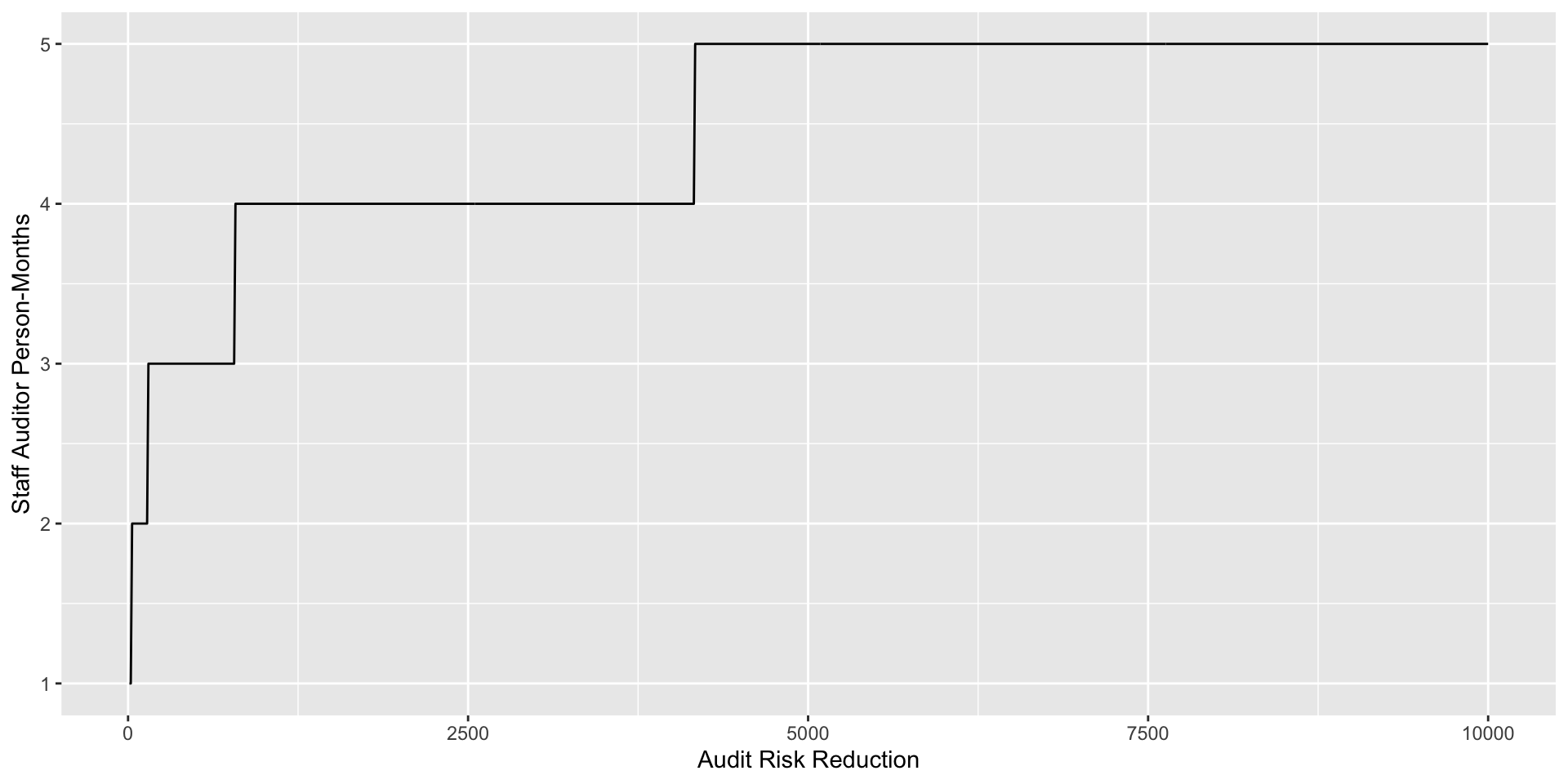
The Risk Assessment Matrix

• A Risk Assessment Matrix is constructed prior to and during the analytical review phase of the audit (see Fig. 2 for an example of a RAM dashboard).
• During this phase, the auditor will scan any business intelligence from media and Internet sources that would be relevant to potential risks to be encountered in the audit of the client. Prior years’ working papers will also be perused for ascertain experiences, client specific risks, and application of the “rule of 3’s” to adjust any anticipated risks and expectations during the current year audit.

リスク評価マトリクスは、監査の分析的手続の前段階およびその実施中に 作成される（RAMダッシュボードの例については、図 2を参照）。 この段階において、監査人は、メディアやインターネット上の情報源から、当該被監査会社の監査で遭遇する潜在的なリスクに関連するビジネス情報を調べ上げる。ま た、過年度の監査調書を閲覧し、経験やクライアント固有のリスクを確認し、「3つの法則（rules of three）」を適用して、当年度の監査で想定されるリスクや 予想事項を調整する。

• Audit firms tend to enforce firm specific procedures in auditing.
• Each of the “Big 4” audit firms displayed unique biases in rendering adverse attestations:
  • Ernst and Young focused on accounts receivables, revenue recognition, taxes, and fixed assets;
  • PricewaterhouseCoopers focused on accounts receivables, revenue recognition, taxes, and payables;
  • KPMG focused on accounts receivables, revenue recognition, taxes, and inventory; and
  • Deloitte and Touche focused on revenue recognition, taxes, liabilities, inventory, and executive compensation (Cheffers 2012).

監査事務所は、監査事務所特有の手続を実施する傾向がある。（米国証券取引所の上場企業のほとんどを監査している）4大監査事務所は、不適正意見を行う際にそれぞれ独自の傾向がある。 それぞれ、EY監査事務所（Ernst & Young）は売掛金、収益認識、税金、および固定資産、 PwC監査事務所（PricewaterhouseCoopers）は売掛金、収益認識、税金、および買掛金、 KPMG監査事務所は売掛金、収益認識、税金、および棚卸資産、 Deloitte監査事務所（Deloitte & Touche）は収益認識、税金、負債、棚卸資産、および役員報酬に重点を置いている（Cheffers 2012）。

• These biases are likely to reflect signature audit methods, internal forms and checklists, and audit histories that are unique to individual firms.
• These firms will consequently allocate larger portions of the audit budget to certain accounts at the expense of others.
• Additionally, auditors tend to allocate more time to auditing debit balance accounts, assuming double-entry will assure the accuracy of the credit accounts.
• The specific accounts selected for audit depend on firm policy, procedures, and managing partners.

このような監査事務所は、その結果、監査予算の多くを特定の勘定科目に割り当て、他の勘定科目を犠牲にすることになる。 さらに、監査人は、複式簿記の法則により貸方勘定の正確性を確保するために、借方勘定残高の監査に多くの時間を割く傾向がある。 監査対象として選択される勘定科目は、監査事務所の方針、手続、パートナーによって異なる。

• In this section, I will show how to construct a Risk Assessment Matrix on a client–server dashboard.
• Dashboards are well suited to auditing—they accommodate the information needs of auditors (and their laptops) in the field, while assuring the security, integrity, completeness, and privacy of client and audit records behind firewalls.
• The Risk Assessment Matrix will assume we are planning the audit of the simulated system presented in chapter “Simulated Transactions for Auditing Service Organizations” (Fig. 2).

本節では、クライアントサーバーのダッシュボード上でリスク評価マトリクスを作成する方法を紹介する。client-serverはクライアントサーバー ダッシュボードは監査に適している。ファイアウォールの背後にある被監査会社と監査調書記録のセキュリティ、一貫性、完全性、およびプライバシーを保証しながら、現場の監査人（とそのノートパソコン）の情報ニーズに対応する。 後にシステムの監査を行っていると仮定した場合のリスク評価マトリクスを示す。

Using Shiny to create a Risk Assessment Matrix Dashboard

RAM

• Auditors face a particular problem in the field, in that much of the information they need may be in prior years’ workpapers, in proprietary client files, in central locations in the audit firm and on powerful servers or cloud platforms.
• The standard solution to such problems is found in client–server systems that place secure systems on a centralized server, and provide the field auditor with light, client software that runs on a laptop, communicating with the server over the Internet.
• Shiny is the client–server extension of the R, and as with the rest of the R, is uniquely suited to handling the ad hoc nature of audits, where each audit often represents an entirely new set of analyses.

Shiny App

• Shiny is a tool for fast prototyping of digital dashboards, giving you a large number of HTML Widgets at your disposal which lend themselves really well to building general-purpose web applications.
• Shiny is particularly suited for fast prototyping and is fairly easy to use for someone who is not a programmer. Dashboards locally display some data (such as in a database or a file) providing a variety of metrics in an interactive way.

Create a RAM Dashboard

• Reactive programming starts with reactive values that change in response to user input and builds on top of them with reactive expressions that access reactive values and execute other reactive expressions.
• Reactivity based code for the Risk Assessment Matrix dashboard appears below.
• This has two parts:
  1. the user interface “ui” which conceivably would operate on the field auditor’s laptop, and
  2. the server-side “server” operations that would take place at the audit firms headquarters and with access to firm and client files.

リアクティブプログラミング（Reactive programming）は、ユーザーの入力に反応して変化するリアクティブ値（信頼度スライダーやコストスライダーの位置決めなど）から始まり、リアクティブ値に反応して他のリアクティブ表現を実行するリアクティブ表現によりダッシュボードの良く見える場所に作成される。 リスク評価マトリクス・ダッシュボードのリアクティブベースのコードを以下で示す。2つの部分から構成されている。 すなわち、(1)現場の監査人のノートパソコンで動作すると考えられる「ユーザインタフェース（user interface：UI）」、および(2)ファイアウォールで保護された監査事務所の本部で行われ、監査事務所と被監査会社のファイルにアクセスできるサーバサイドの「サーバ（server：server）」操作である。まず、ユーザーインターフェースを見てみよう。

Shiny App

# Define UI for application
library(shiny) # Load the shiny package

ui <- fluidPage(
    titlePanel("Risk Assessment Matrix"),
    sidebarLayout(
        sidebarPanel(
            # Input: 監査テストの統計的信頼水準
            sliderInput("confidence", "Confidence:",
                        min = .7,
                        max = .999,
                        value = .95),
            # Input: サンプル取引ごとの監査コスト
            sliderInput("cost", "Audit $ / transaction:",
                        min = 0,
                        max = 500,
                        value = 100),
            # Input: Text for providing a caption for the RAM
            textInput(
                inputId = "caption",
                label = "クライアント:",
                value = "XYZ Corp.")
        ),
        # Main panel for displaying outputs
        mainPanel(
            # Output: slider values entered
            tableOutput("values"),
            # Output: Formatted text for caption
            h3(textOutput("caption", container = span)),
            # Output: total cost of the audit
            textOutput("view"),
            # Output: RAM summary with sample sizes (scope) and cost
            verbatimTextOutput("summary"),
            h6("リスク選択: 1 = 低, 2 = 中, 3 = 高"),
            h6("リスク知能 = ビジネス・インテリジェンス・スキャンニングで示されるリスク水準"),
            h6("前年度リスク = 前期に監査人が示したリスク水準"),
            h6("Scope = estimated discovery sample size that will be needed in the audit of this account"),
            h6("Audit cost = audit labor dollars per sampled transaction"),
            h6("Confidence = statistical confidence"),
            h6("Account Amount and the Ave. Transaction size are in $ without decimals or 000 dividers")
        )
    )
)

• The mathematics of scope assessment takes place on the server.
• I used a very simple “discovery sampling” inspired model (see chapter “Design of Audit Programs”) to compute audit scope which I interpret as sample sizes for various transaction flows, computed as:

n \approx \frac{log(1-confidence)}{log(1-\frac{10-risk_{intelligence} \times risk_{prior}}{100})}

• These are dynamically (reactively in the Shiny vernacular) updated for changes in confidence level and transaction auditing costs established by the auditor.
• A total audit cost of field tests is computed, to be incorporated into the overall budget of the audit.

確率の補足

• この式は、二項分布に基づく発見サンプルサイズ (discovery sample size)」を計算するための公式で，二項分布とはあるイベントが n 回の試行の中で何回発生するかを表す確率分布
• 成功確率をpとしたとき、試行回数 n の中で少なくとも1回そのイベントが発生する確率を求める。
• サンプリングにおいて問題となるのは、「ある許容誤差率」以上のエラーが存在するかどうかを確認するために、どれだけのサンプルサイズを用意すればよいか、という点
• この場合、誤り率 p = 0.05 であり、これを発見するために必要なサンプルサイズ n を求めています。

少なくとも1つの誤りを見つける確率

あるサンプルサイズ n を持ち、誤り率が p = 0.05 であると仮定

1. 誤りが1つも見つからない確率: 各サンプルで誤りが発生しない確率は1 - pで，nの全てにおいて誤りが1つも発生しない確率は(1 - p)^n

2. 少なくとも1つの誤りが見つかる確率:

   • 少なくとも1つの誤りが発生する確率は、1から「誤りが1つも見つからない確率」を引いたもの。1 - (1 - p)^n

3. 信頼水準\text{confidence}: 「少なくとも1つの誤りを検出できる確率」が信頼水準\text{confidence}以上であるために必要なサンプルサイズnを計算 1 - (1 - p)^n = \text{confidence}

サンプルサイズnを求める

サンプルサイズnを解く。両辺から1を引いて整理して，対数をとる。 \begin{aligned} (1 - p)^n &= 1 - \text{confidence}\\ \log((1 - p)^n) &= \log(1 - \text{confidence})\\ n \log(1 - p) &= \log(1 - \text{confidence}) \end{aligned}

n を求めるために、両辺を \log(1 - p) で割ると， n = \frac{\log(1 - \text{confidence})}{\log(1 - p)}

許容誤差率p = 0.05と信頼水準\text{confidence} = 0.95を使うと次のようになる。 n = \frac{\log(1 - 0.95)}{\log(1 - 0.05)}

この計算結果は、発見サンプルサイズnを示しており、監査などにおいて設定された許容誤差率（5%）を 95% の確信で検出するために必要なサンプル数を表している。 この式は、二項分布に基づき「少なくとも1つの誤りを検出する確率が信頼水準\text{confidence}に達するために必要なサンプルサイズn」を計算するためのものです。

Shiny App (Server)

server <- function(input, output) {
    ram <- read.csv(system.file("extdata",
        "risk_asst_matrix.csv",
        package = "auditanalytics",
        mustWork = TRUE)
        )

    sliderValues <- reactive({
        data.frame(
            Audit_Parameter = c("confidence", "cost"),
            Value = as.character(c(input$confidence, input$cost)),
            stringsAsFactors = FALSE)
        })

    output$values <- renderTable({
        sliderValues()
        })

    output$caption <- renderText({
        input$caption
        })

    output$summary <- renderPrint({
        ram <- ram
        conf <- input$confidence
        cost <- input$cost
        risk <- (10 - (as.numeric(ram[,2]) * as.numeric(ram[,3])) )/100
        Scope <-  ceiling( log(1-conf) / log( 1- risk))
        ram <- cbind(ram[,1:5], Scope)
        Min_cost <- Scope * cost
        ram <- cbind(ram[,1:6], Min_cost)
        ram
        })

    output$view <- renderText({ # 監査費用を表示
        ram <- ram # リスク評価行列を読み込む
        conf <- input$confidence # 監査の信頼度
        cost <- input$cost # 監査費用
        risk <- (10 - (as.numeric(ram[,2]) * as.numeric(ram[,3])) )/100 # リスク
        Scope <-  ceiling( log(1-conf) / log( 1- risk)) # 範囲
        ram <- cbind(ram[,1:5], Scope) # リスク評価行列に範囲を追加
        Min_cost <- Scope * cost # 最小監査費用を計算
        minimum_audit_cost <- sum(Min_cost) # 最小監査費用を合計
        c("Minimum estimated audit cost = ",minimum_audit_cost) # 最小監査費用を表示
        })
}

R Studio gives you various options for assembling Shiny apps, including apps with server side code resident on either an RStudio or a bespoke server, and stand-alone client side apps which can be constructed with the following code.

shinyApp(ui = ui, server = server)

Shiny applications not supported in static R Markdown documents

Generating the Audit Budget from the Risk Assessment Matrix

Audit Budgets

• The Risk Assessment Matrix (RAM) will generate qualitative measures of risk along with initial estimates of minimum (discovery) sample sizes.
• This will generally not be sufficient to accurately budget the audit, since higher risk accounts will require audit scope beyond mere “discovery” of errors.

In addition, planning will need to estimate costs associated with:

1. Estimating the rates of errors from control weaknesses of all specific types (in interim tests),
2. Assessing the existence and amount of errors in trial balance accounts (in substantive tests), and
3. Generally assessing structural and qualitative problems in financial information consolidation and presentation.

• The third item is beyond the scope of simple technical metrics, and will require the experience and judgment of audit managers.
• It can probably best be estimated by reviewing prior years’ budgets and assuming similar costs for the current year audit.
• The first two items, though, can be budgeted through a relatively simple linear model with assumptions which reflects the cost structure of a particular audit firm.
• Though each RAM will be auditor and client specific, the prior interactive RAM software can easily be programmed to incorporate such a linear model.

Technical Sampling Structure of the Audit Program

• The technical tests of internal control (interim testing) and account balances (substantive testing) consist of audit work investigating the items in transaction samples.
• The unit of audit work is a sampled transaction, and each type of transaction will be subject to misaccounting through a variety of control weaknesses.

Example : salse transaciton

• A sale could be recorded at the wrong amount, or the wrong item sold could have been recorded, or the sale could have been shipped to the wrong customer, or be recorded in the wrong period.
• Each of these problems reflect a specific audit risk, control weakness, and audit procedure.
• Auditors’ concern with such errors differs in the interim and substantive tests.
• Where this rate suggests a control weakness is significant, the auditor needs to expand the scope of substantive auditing of account balances that are affected by the control weakness.

• Placing these considerations in a more formal mathematical setting, let T_{i,j} represent a particular control weakness j in transaction type i.
• Let S_{i,j} be the interim testing sample size suggested by the RAM to test for control weakness j in transaction type i.
• Let C_{i,j} be the audit cost to test for control weakness j in a single transaction of type i.

Then a simple linear cost model would be:

\text{total cost of technical interim test} = \sum _{i,j} S_{i,j} \times C_{i,j}

The matrix form is typically more useful in writing R language code, because the transaction, cost, and sample values are matrices that can directly use the fast BLAS/LAPACK implementations in R for linear algebra, rather than coding slow, messy, nested for statements. The matrix form is:

\text{total cost of technical interim test} = 1_{(i)}^{\top} \times \left (T \times S^{\top} \times C \right ) \times 1_{(j)}

where 1_{(i)}^{\top} is the row i-vector whose entries are all 1’s, 1_(j) is the column j-vector whose entries are all 1’s, T = \{T_{i,j} \}, S = \{ S_{i,j} \}, and C = \{ C_{i,j} \}.

行列形式は、遅くて面倒な入れ子になったfor文をコーディングするよりも、R言語のコードを書く際には通常より有用である。なぜならば、取引、コスト、およびサンプルの値は行列であり、線形代数のためのRの高速なBLAS/LAPACK実装を直接使うことができるからである。行列の形式は以下の通りである。 ここで、1_{(i)}^Tは要素がすべて1のi行ベクトル、1_(j)は要素がすべて1のj列のベクトル、T = \{T_{i,j} \}、S = \{ S_{i,j} \}、C = \{ C_{i,j} \}である。

Sample Sizes for Budgeting

There are two types of sampling in interim tests:

1. Discovery sampling for discovery of out-of-control transaction streams
2. Attribute sampling for estimating transaction error rate

Discovery sampling sets a sample size that is likely to discover at least one error in the sample if the actual transaction error rate exceeds the minimum acceptable error-rate (alternatively called the out-of-control* rate of error). Discovery tests helps the auditor decide whether the systems processing a particular transaction stream are in or out of control.

許容逸脱率とは、母集団において不備の発生が許容される割合の上限値となり、内部統制の実施基準では前述の通り10%未満となります。 内部統制の実務上は、実施基準上、90%以上の信頼性確保が必要となるため、許容逸脱率は9%が上限です。

発見サンプリングは、目標となるエラー水準を固定して行うサンプリングである。 目標エラー割合は０％かそれに近く設定されるため１件のエラー発見時に目標未達が確定するので、テストは停止される。

• Budgeted sample sizes in interim testing will depend on whether the RAM suggests that control risk is low or high.
• If it is low, then the discovery sample size plus a ‘security’ factor for cases where error is discovered will estimated the scope of auditing.

運用評価手続におけるサンプルサイズの予算は、リスク評価マトリクスにおいて統制リスクが低い/高いことを示唆しているかによって決定する。 リスクが低い場合には、監査の範囲は、発見サンプリングにおけるサンプルサイズに、逸脱が発見された場合の「安全性（security）」ファクターを加えたものによって推定される。

confidence <- seq(.99, 0.7, -0.01) # 0.99から0.7まで0.01刻みのベクトル
n <- (log(1 - confidence)) / log(1 - 0.05) # 発見サンプルサイズを計算
plot(confidence,n, type="l") # 発見サンプルサイズをプロット

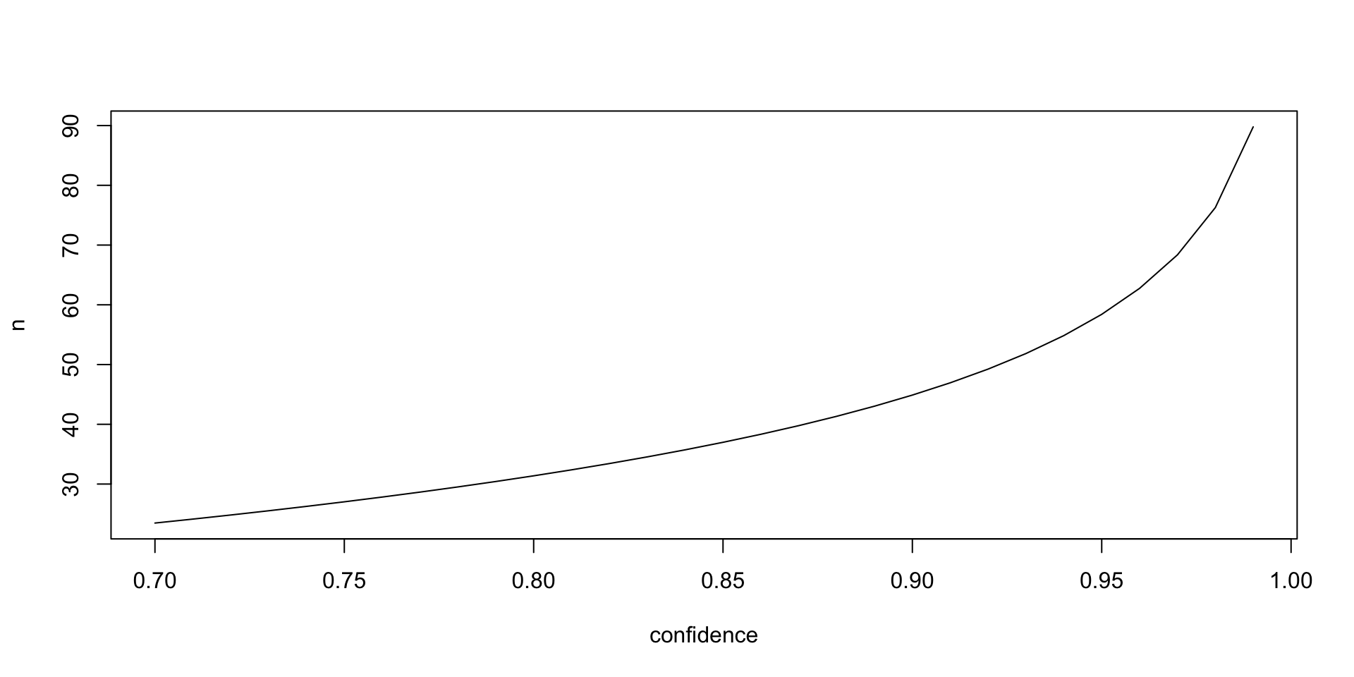
So for a 5% intolerable error rate at 95% confidence we have:

confidence <- 0.95
n <- (log(1 - confidence)) / log(1 - 0.05)
cat("\n Discovery sample size = ", ceiling(n))

 Discovery sample size =  59

Where the RAM assesses control risk to be anything higher, the auditor can assume that scope will be expanded to include attribute sampling.

リスク評価マトリクスが統制リスクをより高く評価する場合には、監査人は、属性サンプリングを実施する範囲を拡大することを前提とする可能性がある。

ここでの log(1 - confidence) と log(1 - 0.05) は、それぞれ信頼水準と許容誤差率を基に、どれだけのサンプルが必要かを対数で計算しています。 これは「二項分布」を利用した計算方法であり、ある確率（この場合、許容誤差率が5%）のイベントが95%の確信で検出されるために必要なサンプル数を算出しています。

• Attribute sampling estimates the error rate in the entire transaction population with some confidence (e.g., 95%) that the estimate is within the out-of-control error-rate cutoff for that transaction stream.
• If it is found that a particular transaction stream is out of control, then attribute estimation will help us decide on the actual error rate of the systems that process this transaction stream.
• If discovery sampling suggests that a particular transaction stream is out of control, then attribute estimation will help us decide on the actual error rate of the systems that process this transaction stream.
• Errors estimates from attribute samples may either be rates or amounts or both.

属性サンプリングは、ある信頼度（例えば95％）により、母集団である取引全体における逸脱率を推定する。 ここで信頼度は、その推定値が当該取引ストリームの許容逸脱率（閾値）以内であることに関するものである。 （発見サンプリングにより）特定の取引ストリームが統制から逸脱していることが判明した場合、属性推定はこの取引ストリームを処理するシステムの実際の逸脱率を決定するのに役立つ。属性サンプルから推定される逸脱は、逸脱率または逸脱数のいずれか、あるいは両方である。 （発見サンプリングにより）特定の取引ストリームが統制から逸脱していることが判明した場合、属性推定はこの取引ストリームを処理するシステムの実際の逸脱率を決定するのに役立つ。 属性サンプルから推定される逸脱は、逸脱率または逸脱数のいずれか、あるいは両方である。

Attribute sampling size is determined using Cohen’s power analysis (Cohen 1992) which is implemented in R’s pwr package, We compute both in the following code chunk

# install.packages("pwr") # first time only
library(pwr)　# Cohen本のpower analysis
size <- 1000 # トランザクションの総数
Delta <- 0.05 * size # 5%の許容エラー率を検出する
sigma <- 0.3 * size # 変動（おそらく1/3）を推測する
effect <- Delta/sigma # 許容度÷変動
sample <- pwr.t.test( # pwr.t.test関数を使用
    d = effect, sig.level = 0.05, power = 0.8,
    type = "one.sample",
    alternative = "greater" ## look for overstatement of earnings
    )
cat("\n Attribute sample size for occurrence of error = ", ceiling(sample$n))

 Attribute sample size for occurrence of error =  224

Attribute sampling determines sample size to estimate the error amount in a transaction stream.

size <- 100000     ## total amount of transactions
mu <- 50           ## average value of transaction
Delta <- 0.05 * mu ## detect 5% amount intolerrable error
sigma <- 30        ## variability
effect <- Delta/sigma
sample <- pwr.t.test(
  d = effect, sig.level = 0.05, power = 0.8,
  type = "one.sample", alternative = "greater")
cat("\n Attribute sample size for amount of error = ", ceiling(sample$n))

 Attribute sample size for amount of error =  892

• The auditor faces different decisions in substantive testing.
• The particular type of account determines the impact of control weaknesses found in interim testing.
• For example, a 5% error rate in a $1 million sales account discovered in interim testing implies a $50,000 error in annual sales on the trial balance.
• Assume that accounts receivable turn over 10 times annually, then that 5% error rate implies only a $5000 misstatement in accounts receivable.
• Whether sales or accounts receivable are ‘fairly stated’ depends on the immateriality level set by the auditor – a $10,000 materiality level would imply that sales is not fairly presented, while accounts receivable is fairly stated.

• At year-end where there will be a complete set of transactions available for the year, and substantive samples are typically focused on acceptance sampling to determine of the account balance is ‘fairly stated’ (does not contain intolerable or material error).
• The approach is the same as attribute sampling of amounts, and is inherently more straightforward than interim control tests.
• Substantive tests estimate the error rate in an account balance with some confidence (e.g., 95%) that the estimate is within the ‘materiality’ or ‘intolerable error’ cutoff for that account balance

• For example, consider sampling sales invoices from the accounts receivable aging report and comparing them to supporting documentation to see if they were billed in the correct amounts, to the correct customers, and on the correct dates.
• Additionally, auditors might trace invoices to shipping log, and match invoice dates to the shipment dates for those items in the shipping log, to see if sales are being recorded in the correct accounting period.
• This can include an examination of invoices issued after the period being audited, to see if they should have been included in a prior period.

• Acceptance sampling size is determined using Cohen’s power analysis which is implemented in R’s pwr package, If discovery sampling suggests that a particular transaction stream is out of control, then attribute estimation will help us decide on the actual error rate of the systems that process this transaction stream.
• Errors estimates from attribute samples may either be rates of erroneous transactions or from a monetary unit sampling perspective, can be rates of monetary error in the transaction stream.

We compute both in the following code chunk

size   <- 100000      # 取引の総額
mu     <- 50          # 取引の平均値
Delta  <- 0.05 * mu   # 5%の金額の許容誤差を検出
sigma  <- 30          # 変動
effect <- Delta / sigma # 許容度÷変動

sample <- pwr.t.test( # Cohenのpower analysis
  d = effect,       # Cohenのd
  sig.level = 0.05, # 有意水準
  power = 0.8,      # 効果量
  type = "one.sample", # 一標本検定
  alternative = "greater" # 偽陽性
  )
cat("\n Attribute sample size for amount of error = ", ceiling(sample$n))

 Attribute sample size for amount of error =  892

Notable Audit Failures and Why They Occurred

• Audit and accounting practice have been strongly influenced by a string of scandals that have occurred nearly every 7 years since the Reagan reforms of the early 1980s.
• The medical, legal and accounting professions were opened up to free-market forces when all three professions were allowed direct-to-consumer marketing and brand-building.
• Rules regarding pricing and competition for talent were also relaxed.

監査実務と会計実務は、1980年代初頭のレーガン改革以来、ほぼ7年ごとに発生している一連のスキャンダルに強く影響を受けてきた。 医療、法律、会計の各専門職は、直接消費者向けのマーケティングとブランド構築が許可されたとき、自由市場の力によって開かれた。 価格設定や人材の競争に関する規則も緩和された。

• In auditing the repeal of AICPA Ethics Rules Section 501 on advertising, recruiting from other firms and other free-market innovations moved the industry from its cossetted clubby culture to a profit-oriented business. − By the late 1990s audit firms were averaging $7 of IT revenue for every $1 of audit revenue.
• The year 2001 witnessed a series of financial frauds involving Enron Corporation auditing firm Arthur Andersen, the telecommunications company WorldCom, Qwest, and Sunbeam among other well-known corporations.

監査において、AICPA倫理規則第501条（広告、他の企業からの採用など）の廃止、他の企業からの採用などの自由市場の革新により、業界は、保護されたクラブ文化から利益志向のビジネスへと移行した。 1990年代後半には、監査会社は監査収益1ドルに対してIT収益7ドルを平均していた。 2001年には、エンロン社、監査会社アーサー・アンダーセン、通信会社ワールドコム、クエスト、サンビームなどの他の有名な企業を巻き込んだ一連の財務詐欺事件が発生した。

• These problems highlighted the need to review the effectiveness of accounting standards, auditing regulations and corporate governance principles.
• In some cases, management manipulated the figures shown in financial reports to indicate a better economic performance.
• In others, tax and regulatory incentives encouraged over-leveraging of companies and decisions to bear extraordinary and unjustified risk.

これらの問題は、会計基準、監査規制、企業ガバナンス原則の有効性を見直す必要性を浮き彫りにした。 一部の場合、経営陣は財務報告書に表示される数字を操作して、より良い経済的成績を示そうとした。 他の場合、税制や規制上のインセンティブが企業の過剰レバレッジや非常識なリスクを負う決定を促した。

• The Enron scandal deeply influenced the development of new regulations to improve the reliability of financial reporting and increased public awareness about the importance of having accounting standards that show the financial reality of companies and the objectivity and independence of auditing firms.
• In addition to being the largest bankruptcy reorganization in American history, the Enron scandal undoubtedly is the biggest audit failure. The scandal caused the dissolution of Arthur Andersen which at the time was one of the five largest accounting firms in the world.
• One consequence of these events was the passage of the Sarbanes–Oxley Act in 2002.

エンロンの不祥事は、会計基準が企業の財務の実態を示し、監査会社の客観性と独立性を示すことの重要性についての公衆の認識を高めるための新しい規制の開発に大きな影響を与えた。 アメリカ史上最大の破産再編であるだけでなく、エンロンの不祥事は間違いなく最大の監査失敗である。 この不祥事は、当時世界で5番目に大きな会計事務所の1つであったアーサー・アンダーセンの解散を引き起こした。 これらの出来事の一つの結果は、2002年にサーベインズ・オクスリー法が成立したことである。 この法律は、連邦捜査で記録を破壊、変更、または偽造し、株主を詐欺しようとするあらゆる計画や試みに対する証券詐欺の刑事罰を大幅に引き上げている。

Auditing: A Wicked Problem

Wicked Problem

• In theory, independent audits increase the value and credibility of the financial statements, reduce investor risk, and reduce the cost of capital of audited firms.
• They are often required under securities law and by investors and creditors.
• But such assertions have grown increasingly contentious over time as the definitions and usage of financial statements have evolved and changed.
• Scholars are increasingly aware that many of auditing’s difficulties reflect its status as a wicked problem.

理論上では，独立した監査は，財務諸表の価値と信頼性を高め，投資家のリスクを低減し，監査対象企業の資本コストを低減する。 これらは，証券法によって要求されることが多く，投資家や債権者によっても要求される。 しかし，これらの主張は，財務諸表の定義や使用法が進化し変化するにつれて，ますます論争の的となってきている。 学者たちは，監査の多くの困難が，それが悪い問題であるという状況を反映していることにますます気づいている。

• Wicked problems are difficult or impossible to solve because of incomplete, contradictory and changing requirements that are often difficult to recognize.
• The term wicked is used not in the sense of evil but rather its resistance to resolution.
• Moreover because of complex interdependencies, the effort to solve one aspect of a wicked problem may reveal or create other problems.
• Contrast this with relatively tame soluble problems in mathematics, chess or puzzle solving (Coyne 2005; Ludwig 2001; Rittel and Webber 1973).

悪い問題は，不完全で矛盾した要件や変化する要件によって解決が困難または不可能であり，これらの要件はしばしば認識が難しい。 「悪い」という用語は，悪意のあるという意味ではなく，むしろ解決に対する抵抗という意味で使われている。 さらに，複雑な相互依存関係のため，悪い問題の一つの側面を解決しようとする努力は，他の問題を明らかにしたり作り出したりするかもしれない。 これに対して，数学，チェス，パズル解決などの比較的穏やかな解決可能な問題とは対照的である（Coyne 2005; Ludwig 2001; Rittel and Webber 1973）。

Wicked Problems

• Audits are classic wicked problems sharing the following characteristics (Rittel and Webber 1973):

1. There is no definitive formulation of auditing.
2. Audits have no stopping rule.
3. Audit products are not true-or-false rather are opinions.
4. There is no immediate and no ultimate test of an audit conclusion.
5. Each audit is a one-shot operation.

監査は、次の特徴を共有する古典的な「悪い問題」である（Rittel and Webber 1973）。

1. 監査の明確な定式化がない。
2. 監査には停止規則がない。
3. 監査の成果物は真偽ではなく意見である。
4. 監査の結論には即時テストも最終テストもない。
5. 各監査は一回限りの作業である。

6. Audits do not have an enumerable or an exhaustively describable set of potential solutions nor is there a well-described set of permissible operations that may be incorporated into the audit program.
7. Every audit is essentially unique.
8. Every audit procedure can be considered to be a response to some other finding.
9. The existence of an audit discrepancy can be explained in numerous ways. The choice of explanation determines the nature of the problems resolution and the audit opinion.

6. 監査には、列挙可能な、あるいは網羅的に記述可能な潜在的解決策の集合があるわけではなく、また監査プログラムに組み込むことができる許容される操作のセットも存在しない
7. すべての監査は本質的に一意である。
8. すべての監査手続は他の発見事項に対する対応であると考えることができる。
9. 監査上の不一致の存在は、多くの方法で説明することができる。どの説明を選択するかによって、問題解決と監査意見の性質が決まる。説明の選択により、問題解決と監査意見の性質が決まる。

10. The auditor has no right to be wrong and is ultimately liable for the consequences of audit opinions.
11. The solution depends on how the problem is framed and vice versa, i.e., the problem definition depends on the solution.
12. Stakeholders have radically different world views and different frames for understanding the problem.
13. The constraints that the problem is subject to and the resources needed to solve it change over time.

10. 監査人は監査意見を誤る権利を有しておらず、監査意見の結果について最終的な責任を負う。
11. つまり問題の定義が解決策に依存している。
12. 利害関係者は、根本的に異なる世界観を持っており、問題を理解するためのフレームも異なる。
13. 問題の対象となる制約や、解決に必要な資源は、時間とともに変化する。 –>

Competitive Strategies

• Roberts (2002) and Roberts (2000) identified three strategies to address wicked problems: competitive, authoritative and collaborative.
• Competitive strategies attempt to solve wicked problems by pitting opposing points of view against each other requiring parties that hold these views to come up with their preferred solutions.
• The advantage of this approach is that different solutions can be weighed up against each other and the best one chosen.
• The disadvantage is that this adversarial approach creates a confrontational environment in which knowledge sharing is discouraged.

Collaborative Strategies

• Collaborative strategies try to engage all stakeholders in order to find the best possible solution for all stakeholders.
• Typically these approaches involve meetings in which issues and ideas are discussed and a common agreed approach is formulated.
• Such approaches share many of the disadvantages of competitive approaches and can be even more time consuming.

Authoritative Strategies

• Authoritative strategies concentrate responsibility for solving the problems in the hands of a few people, for example Certified Public Accountants.
• The reduction in the number of stakeholders reduces problem complexity as many competing points of view are eliminated at the start.
• The disadvantage is that authorities and experts charged with solving the problem lack all of the information needed to efficiently and completely solve the problem.

Auditing as a Wicked Problem

• Auditing for better or worse has chosen to couch the industrial organization of the audit business in an authoritarian structure.

• Authority for rendering audit opinions is vested in a small number of firms; the Fortune 500 firms must typically be audited by one of the Big Four audit firms;

• Audits authoritative strategy for solving its wicked problem offers the advantage of substantially reduced cost and greater efficiency of audits.

• Its disadvantage is that no matter how well educated the auditors are they will not have as much information about IT storage and processing platforms.

Final Thoughts on Planning and Budgets

• Planning and budgeting of audits is not an exact science, rather it is contextual, with uncertain outcomes, incomplete and asymmetric information, and ongoing negotiations with the client and between audit offices.
• The judgment and experience of auditors, managers, and the profession are essential to a complete and effective planning process.
• Since audit planning will often be highly collaborative, involving professionals in different offices around the world, computational tools to aid in standardizing and objectifying procedures across languages and cultures can be expected to improve efficiency and effectiveness of auditing.